Download Code

Frequentist Estimation and Bayesian Inference

Chris Slaughter

March 26, 2026

library(rms)
library(ggplot2)
library(plotly)
library(brms)
library(tidyverse)
library(coda)
library(MASS)
library(truncnorm)
library(knitr)
library(kableExtra)

1 Introduction

These notes provide a comparison of Frequentist Estimation and Bayesian Inference approaches to regression modeling. This material is presented as one of the final lectures before the exam and builds upon foundational concepts covered in earlier course materials.

Prerequisites: Before working through these notes, we will first review Model Estimation (Set2.pdf), which covers key concepts in simple linear regression and details on estimation from a frequentist standpoint. That material provides a review of many applied concepts already discussed (and thus serves as a review for the midterm exam) and is the foundation for understanding the comparisons presented here.

Scope and Purpose: These following notes present mathematical derivations and theoretical foundations to provide clarity and deeper understanding of both approaches. The derivations demonstrate in linear and logistic regression

• How maximum likelihood estimation works

• How Bayesian posterior distributions are derived

• The relationship between different estimation methods

• The underlying theory behind the functions you use in practice

Important Note on Exam Coverage:

The exam focuses on applied data analysis. While the mathematical derivations in these notes are provided for clarity and understanding, in this course you are NOT be asked to:

• Derive posterior distributions

• Maximize likelihood functions by hand

• Perform calculus-based derivations

These derivation skills are the purview of other courses. For this course, you should focus on:

• Understanding the conceptual differences between approaches

• Knowing when to use each method

• Applying the methods using R (lm(), glm(), brms(), etc.)

• Interpreting and communicating results

2 Linear Regression

We consider a simplified linear regression model with only a slope parameter (no intercept) with \(X_i\) fixed. This model takes the form:

\[Y_i = \beta X_i + \varepsilon_i\]

where \(\varepsilon_i \sim N(0, \sigma^2)\) for the likelihood-based approach.

Important Note: This model forces the regression line through the origin \((0,0)\). While mathematically simpler (reducing the parameter space), this constraint is often not scientifically useful. Even if we expect \(Y=0\) when \(X=0\), this point may lie outside the range of our data and assumes linearity, making the constraint arbitrary and potentially misleading.

2.1 Frequentist Estimation

2.1.1 Maximum Likelihood Estimation

The maximum likelihood approach assumes conditional normality of the residuals. Given \(Y_i \sim N(\beta X_i, \sigma^2)\), the likelihood function is:

\[L(\beta, \sigma^2 | \mathbf{y}, \mathbf{x}) = \prod_{i=1}^n \frac{1}{\sqrt{2\pi\sigma^2}} \exp\left(-\frac{(y_i - \beta x_i)^2}{2\sigma^2}\right)\]

The log-likelihood is:

\[\ell(\beta, \sigma^2) = -\frac{n}{2}\log(2\pi) - \frac{n}{2}\log(\sigma^2) - \frac{1}{2\sigma^2}\sum_{i=1}^n(y_i - \beta x_i)^2\]

Deriving the MLE for \(\beta\):

Taking the derivative with respect to \(\beta\) and setting equal to zero:

\[\frac{\partial \ell}{\partial \beta} = \frac{1}{\sigma^2}\sum_{i=1}^n x_i(y_i - \beta x_i) = 0\]

\[\sum_{i=1}^n x_i y_i - \beta \sum_{i=1}^n x_i^2 = 0\]

\[\hat{\beta}_{MLE} = \frac{\sum_{i=1}^n x_i y_i}{\sum_{i=1}^n x_i^2}\]

Deriving the MLE for \(\sigma^2\):

Taking the derivative with respect to \(\sigma^2\):

\[\frac{\partial \ell}{\partial \sigma^2} = -\frac{n}{2\sigma^2} + \frac{1}{2\sigma^4}\sum_{i=1}^n(y_i - \beta x_i)^2 = 0\]

\[\hat{\sigma}^2_{MLE} = \frac{1}{n}\sum_{i=1}^n(y_i - \hat{\beta} x_i)^2\]

2.1.1.1 Standard Error via Fisher Information

The Fisher Information matrix provides the asymptotic variance of the MLE. For our model:

\[I(\beta, \sigma^2) = -E\left[\frac{\partial^2 \ell}{\partial \theta \partial \theta^T}\right]\]

The second derivatives are:

\[\frac{\partial^2 \ell}{\partial \beta^2} = -\frac{1}{\sigma^2}\sum_{i=1}^n x_i^2\]

\[\frac{\partial^2 \ell}{\partial (\sigma^2)^2} = \frac{n}{2\sigma^4} - \frac{1}{\sigma^6}\sum_{i=1}^n(y_i - \beta x_i)^2\]

\[\frac{\partial^2 \ell}{\partial \beta \partial \sigma^2} = -\frac{1}{\sigma^4}\sum_{i=1}^n x_i(y_i - \beta x_i)\]

Taking expectations (where \(E[(y_i - \beta x_i)^2] = \sigma^2\) and \(E[y_i - \beta x_i] = 0\)):

\[I(\beta) = \frac{1}{\sigma^2}\sum_{i=1}^n x_i^2\]

Therefore, the asymptotic variance is:

\[\text{Var}(\hat{\beta}) = \frac{\sigma^2}{\sum_{i=1}^n x_i^2}\]

\[SE(\hat{\beta}) = \frac{\sigma}{\sqrt{\sum_{i=1}^n x_i^2}}\]

In practice, we substitute \(\hat{\sigma}\) for \(\sigma\).

Important Note on Bias: The MLE estimate of \(\sigma^2\) is:

\[\hat{\sigma}^2_{MLE} = \frac{1}{n}\sum_{i=1}^n(y_i - \hat{\beta} x_i)^2\]

This estimator is biased because it uses \(n\) in the denominator rather than the degrees of freedom \((n-1)\). The MLE is asymptotically unbiased but has finite-sample bias. To obtain an unbiased estimator of \(\sigma^2\), we use:

\[\hat{\sigma}^2_{unbiased} = \frac{1}{n-1}\sum_{i=1}^n(y_i - \hat{\beta} x_i)^2\]

The correction factor is \(\frac{n}{n-1}\), so:

\[\hat{\sigma}_{unbiased} = \sqrt{\frac{n}{n-1}} \cdot \hat{\sigma}_{MLE}\]

When calculating the standard error of \(\hat{\beta}\), using the unbiased estimator ensures:

\[SE(\hat{\beta}) = \frac{\hat{\sigma}_{unbiased}}{\sqrt{\sum_{i=1}^n x_i^2}} = \frac{\sqrt{\frac{1}{n-1}\sum_{i=1}^n(y_i - \hat{\beta} x_i)^2}}{\sqrt{\sum_{i=1}^n x_i^2}}\]

This matches the standard error reported by lm() exactly.

2.1.1.2 Standard Error via Basic Variance Principles

We can also derive the standard error directly from the formula for \(\hat{\beta}\):

\[\hat{\beta} = \frac{\sum_{i=1}^n x_i Y_i}{\sum_{i=1}^n x_i^2}\]

Since \(Y_i = \beta x_i + \varepsilon_i\) where \(\varepsilon_i \sim N(0, \sigma^2)\) independently:

\[\text{Var}(\hat{\beta}) = \text{Var}\left(\frac{\sum_{i=1}^n x_i Y_i}{\sum_{i=1}^n x_i^2}\right) = \frac{1}{(\sum_{i=1}^n x_i^2)^2} \text{Var}\left(\sum_{i=1}^n x_i Y_i\right)\]

Since the \(Y_i\) are independent:

\[\text{Var}\left(\sum_{i=1}^n x_i Y_i\right) = \sum_{i=1}^n x_i^2 \text{Var}(Y_i) = \sum_{i=1}^n x_i^2 \sigma^2 = \sigma^2 \sum_{i=1}^n x_i^2\]

Therefore:

\[\text{Var}(\hat{\beta}) = \frac{\sigma^2 \sum_{i=1}^n x_i^2}{(\sum_{i=1}^n x_i^2)^2} = \frac{\sigma^2}{\sum_{i=1}^n x_i^2}\]

This confirms our Fisher Information result.

2.1.2 Estimating Equations Approach (Least Squares)

The least squares approach minimizes the residual sum of squares without assuming normality. We minimize:

\[RSS(\beta) = \sum_{i=1}^n (y_i - \beta x_i)^2\]

Taking the derivative and setting to zero:

\[\frac{\partial RSS}{\partial \beta} = -2\sum_{i=1}^n x_i(y_i - \beta x_i) = 0\]

\[\hat{\beta}_{LS} = \frac{\sum_{i=1}^n x_i y_i}{\sum_{i=1}^n x_i^2}\]

Note that \(\hat{\beta}_{LS} = \hat{\beta}_{MLE}\) even though the least squares approach does not require the normality assumption. The normality assumption is only needed for inference (standard errors, confidence intervals, hypothesis tests) in small samples, though large-sample inference can rely on asymptotic normality via the Central Limit Theorem.

2.1.3 Demonstration with Real Data

We’ll use the cars dataset in R, which contains speed and stopping distance for cars.

# Load and prepare data
data(cars)
# We'll model distance as a function of speed with no intercept
y <- cars$dist
x <- cars$speed

# Calculate estimates
beta_hat <- sum(x * y) / sum(x^2)
n <- length(y)
residuals <- y - beta_hat * x
RSS <- sum(residuals^2)

# MLE estimate of sigma (biased)
sigma_hat_mle <- sqrt(RSS / n)

# Unbiased estimate of sigma
sigma_hat_unbiased <- sqrt(RSS / (n - 1))

# Correction factor
correction_factor <- sqrt(n / (n - 1))

# Create comparison table
comparison_df <- data.frame(
  Estimate = c("β̂", "σ̂ (MLE)", "σ̂ (unbiased)", "Correction factor", "SE(β̂) using MLE σ", "SE(β̂) using unbiased σ"),
  Value = c(
    round(beta_hat, 4),
    round(sigma_hat_mle, 4),
    round(sigma_hat_unbiased, 4),
    round(correction_factor, 4),
    round(sigma_hat_mle / sqrt(sum(x^2)), 4),
    round(sigma_hat_unbiased / sqrt(sum(x^2)), 4)
  )
)

kable(comparison_df, caption = "Manual Calculation Results", align = 'll', format='html') %>%
  kable_styling(bootstrap_options = c("striped", "hover"))

Manual Calculation Results

Estimate	Value
β̂	2.9091
σ̂ (MLE)	16.0958
σ̂ (unbiased)	16.2592
Correction factor	1.0102
SE(β̂) using MLE σ	0.1399
SE(β̂) using unbiased σ	0.1414

2.1.3.1 3D Likelihood Surface

Now we’ll create a 3D plot showing the likelihood function as a function of \(\beta\) and \(\sigma\):

# Make sure beta_hat and sigma_hat_mle are on the grid
beta_grid  <- sort(unique(c(seq(beta_hat - 0.5, beta_hat + 0.5, length.out = 50), beta_hat)))
sigma_grid <- sort(unique(c(seq(max(1, sigma_hat_unbiased - 5), sigma_hat_unbiased + 5, length.out = 50), sigma_hat_mle)))

# Compute log-likelihood
log_lik <- outer(beta_grid, sigma_grid, Vectorize(function(beta, sigma) {
  res <- y - beta * x
  n <- length(y)
  -n/2 * log(2*pi) - n * log(sigma) - sum(res^2)/(2*sigma^2)
}))

# Relative likelihood (max = 1 at MLE on the grid)
likelihood <- exp(log_lik - max(log_lik))

# Relative likelihood values at the two sigma points with beta fixed at beta_hat
rel_at <- function(beta0, sigma0) {
  res <- y - beta0 * x
  n <- length(y)
  ll <- -n/2 * log(2*pi) - n * log(sigma0) - sum(res^2)/(2*sigma0^2)
  exp(ll - max(log_lik))
}

z_mle      <- rel_at(beta_hat, sigma_hat_mle)
z_unbiased <- rel_at(beta_hat, sigma_hat_unbiased)

plot_ly(x = ~sigma_grid, y = ~beta_grid, z = ~likelihood) %>%
  add_surface() %>%
  add_markers(x = sigma_hat_mle, y = beta_hat, z = z_mle,
              marker = list(size = 5, color = 'red'),
              name = 'MLE (σ)') %>%
  add_markers(x = sigma_hat_unbiased, y = beta_hat, z = z_unbiased,
              marker = list(size = 5, color = 'blue'),
              name = 'Unbiased (σ)') %>%
  layout(scene = list(
    xaxis = list(title = 'σ'),
    yaxis = list(title = 'β'),
    zaxis = list(title = 'Relative Likelihood')
  ))

The red point shows the MLE estimate \((\hat{\beta}, \hat{\sigma}_{MLE})\), which corresponds to the maximum of the likelihood function. The blue point shows \((\hat{\beta}, \hat{\sigma}_{unbiased})\), which uses the degrees-of-freedom correction. Note that \(\hat{\beta}\) is the same for both (it maximizes the likelihood), but the unbiased estimator of \(\sigma\) is slightly larger.

2.1.3.2 Comparison with lm()

Now let’s verify our results using R’s built-in lm() function:

# Fit model with lm (forcing through origin with -1)
model_lm <- lm(dist ~ speed - 1, data = cars)

# Create comparison table
comparison_lm <- data.frame(
  Estimate = c("β̂", "SE(β̂)"),
  Manual = c(round(beta_hat, 4), round(sigma_hat_unbiased / sqrt(sum(x^2)), 4)),
  `lm()` = c(round(coef(model_lm)[1], 4), round(summary(model_lm)$coefficients[1, 2], 4)),
  check.names = FALSE
)

kable(comparison_lm, caption = "Comparison: Manual Calculation vs lm()", align = 'lrr', format='html') %>%
  kable_styling(bootstrap_options = c("striped", "hover"))

Comparison: Manual Calculation vs lm()

	Estimate	Manual	lm()
speed	β̂	2.9091	2.9091
	SE(β̂)	0.1414	0.1414

The estimates match perfectly, confirming our derivations.

2.2 Bayesian Inference

For the Bayesian approach, we use conditionally conjugate priors. Let \(\tau = 1/\sigma^2\) denote the precision. We specify:

• Prior for \(\beta\): \(\beta \sim N(\mu_0, 1/\tau_0)\)

• Prior for \(\tau\): \(\tau \sim \text{Gamma}(\alpha_0, \beta_0)\)

These priors are conditionally conjugate, meaning each complete conditional distribution has a recognizable form.

2.2.1 Complete Conditional Distributions

Complete Conditional for \(\beta\):

The likelihood contribution is: \[p(\mathbf{y}|\beta, \tau) \propto \exp\left(-\frac{\tau}{2}\sum_{i=1}^n(y_i - \beta x_i)^2\right)\]

The prior is: \[p(\beta) \propto \exp\left(-\frac{\tau_0}{2}(\beta - \mu_0)^2\right)\]

The posterior (using kernel recognition) is: \[p(\beta | \mathbf{y}, \tau) \propto \exp\left(-\frac{1}{2}\left[\tau\sum_{i=1}^n(y_i - \beta x_i)^2 + \tau_0(\beta - \mu_0)^2\right]\right)\]

Background: Kernel Recognition for Posterior Distributions

Kernel recognition is a technique for identifying probability distributions from their unnormalized forms. The key insight is that we can recognize a distribution by its “kernel”—the part that depends on the parameter of interest, ignoring normalizing constants.

2.2.2 The Basic Principle

For a probability density \(p(\theta)\), we can write:

\[p(\theta) = \frac{1}{c} \times k(\theta)\]

where:

• \(k(\theta)\) is the kernel (the part depending on \(\theta\))

• \(c\) is the normalizing constant (makes the integral/sum equal 1)

In Bayesian inference, we compute:

\[p(\theta | \text{data}) \propto p(\text{data} | \theta) \times p(\theta)\]

The \(\propto\) symbol means “proportional to”—we ignore constants that don’t depend on \(\theta\). If we can recognize the resulting kernel as belonging to a known distribution family, we’ve identified the posterior.

2.2.3 Common Kernels to Recognize

Normal Distribution: \(N(\mu, \sigma^2)\)

Kernel: \(\exp\left(-\frac{1}{2\sigma^2}(x - \mu)^2\right)\)

Key pattern: Quadratic in the exponent \[\exp\left(-\frac{1}{2}[\text{constant} \times \theta^2 - 2 \times \text{constant} \times \theta]\right)\]

Gamma Distribution: \(\text{Gamma}(\alpha, \beta)\)

Kernel: \(x^{\alpha-1} e^{-\beta x}\)

Key pattern: Power times exponential

Beta Distribution: \(\text{Beta}(\alpha, \beta)\)

Kernel: \(x^{\alpha-1}(1-x)^{\beta-1}\)

Key pattern: Product of powers

2.2.4 Example: Normal Posterior

Suppose we have:

• Data: \(y_i \sim N(\theta, \sigma^2)\) with known \(\sigma^2\)

• Prior: \(\theta \sim N(\mu_0, \tau_0^2)\)

The posterior is: \[p(\theta | \mathbf{y}) \propto \exp\left(-\frac{1}{2\sigma^2}\sum(y_i - \theta)^2\right) \times \exp\left(-\frac{1}{2\tau_0^2}(\theta - \mu_0)^2\right)\]

Step 1: Expand and combine exponents: \[\propto \exp\left(-\frac{1}{2}\left[\frac{n}{\sigma^2}\theta^2 - \frac{2\sum y_i}{\sigma^2}\theta + \frac{1}{\tau_0^2}\theta^2 - \frac{2\mu_0}{\tau_0^2}\theta\right]\right)\]

Step 2: Collect terms: \[\propto \exp\left(-\frac{1}{2}\left[\left(\frac{n}{\sigma^2} + \frac{1}{\tau_0^2}\right)\theta^2 - 2\left(\frac{\sum y_i}{\sigma^2} + \frac{\mu_0}{\tau_0^2}\right)\theta\right]\right)\]

Step 3: Recognize the pattern \(\exp(-\frac{1}{2}[A\theta^2 - 2B\theta])\) as Normal with:

• Precision: \(\tau_n = \frac{n}{\sigma^2} + \frac{1}{\tau_0^2}\)

• Mean: \(\mu_n = \frac{B}{A} = \frac{\sum y_i/\sigma^2 + \mu_0/\tau_0^2}{n/\sigma^2 + 1/\tau_0^2}\)

Therefore: \(\theta | \mathbf{y} \sim N(\mu_n, 1/\tau_n)\)

2.2.5 The “Completing the Square” Trick

For normal kernels, we often need to complete the square:

Starting with: \(A\theta^2 - 2B\theta + C\)

Rewrite as: \(A(\theta - B/A)^2 + \text{constant}\)

The constant doesn’t depend on \(\theta\), so we can ignore it! This reveals:

• Mean: \(\mu = B/A\)

• Variance: \(\sigma^2 = 1/A\)

2.2.6 Why This Works

The normalizing constant ensures the distribution integrates to 1, but it’s the same for any value of the data. Since we’re conditioning on the observed data, the normalizing constant is just a number that makes the probabilities sum/integrate to 1. We can figure out what distribution we have without computing it!

2.2.7 Practical Tips

1. Expand everything in the posterior expression
2. Collect like terms (all \(\theta^2\) terms together, all \(\theta\) terms together)
3. Ignore constants that don’t involve \(\theta\)
4. Match the pattern to a known distribution
5. Extract parameters from the coefficients

This technique is powerful because it lets us derive closed-form posteriors without doing any integration!

Expanding and completing the square: \[\tau\sum_{i=1}^n(y_i - \beta x_i)^2 + \tau_0(\beta - \mu_0)^2 = (\tau\sum x_i^2 + \tau_0)\beta^2 - 2\beta(\tau\sum x_i y_i + \tau_0\mu_0) + C\]

This is the kernel of a normal distribution: \[\beta | \mathbf{y}, \tau \sim N\left(\frac{\tau\sum x_i y_i + \tau_0\mu_0}{\tau\sum x_i^2 + \tau_0}, \frac{1}{\tau\sum x_i^2 + \tau_0}\right)\]

Let \(\tau_n = \tau\sum x_i^2 + \tau_0\) and \(\mu_n = \frac{\tau\sum x_i y_i + \tau_0\mu_0}{\tau_n}\).

Complete Conditional for \(\tau\):

The likelihood contribution is: \[p(\mathbf{y}|\beta, \tau) \propto \tau^{n/2} \exp\left(-\frac{\tau}{2}\sum_{i=1}^n(y_i - \beta x_i)^2\right)\]

The prior is: \[p(\tau) \propto \tau^{\alpha_0-1} \exp(-\beta_0\tau)\]

The posterior is: \[p(\tau | \mathbf{y}, \beta) \propto \tau^{n/2 + \alpha_0 - 1} \exp\left(-\tau\left[\frac{1}{2}\sum_{i=1}^n(y_i - \beta x_i)^2 + \beta_0\right]\right)\]

This is the kernel of a Gamma distribution: \[\tau | \mathbf{y}, \beta \sim \text{Gamma}\left(\alpha_0 + \frac{n}{2}, \beta_0 + \frac{1}{2}\sum_{i=1}^n(y_i - \beta x_i)^2\right)\]

2.2.8 Gibbs Sampling

Gibbs sampling is a Markov Chain Monte Carlo (MCMC) method that generates samples from a joint posterior distribution by iteratively sampling from complete conditional distributions. The algorithm proceeds as follows:

1. Initialize \(\beta^{(0)}\) and \(\tau^{(0)}\)

2. For iteration \(t = 1, 2, \ldots, T\):

   • Sample \(\beta^{(t)} \sim p(\beta | \mathbf{y}, \tau^{(t-1)})\)

   • Sample \(\tau^{(t)} \sim p(\tau | \mathbf{y}, \beta^{(t)})\)

Under regularity conditions, the samples \((\beta^{(t)}, \tau^{(t)})\) converge to samples from the joint posterior \(p(\beta, \tau | \mathbf{y})\).

2.2.9 Implementation with Diffuse Priors

We’ll use diffuse (weakly informative) priors: - \(\beta \sim N(0, 1000)\) (equivalent to \(\tau_0 = 0.001\), \(\mu_0 = 0\)) - \(\tau \sim \text{Gamma}(0.001, 0.001)\) (equivalent to \(\alpha_0 = 0.001\), \(\beta_0 = 0.001\))

# Gibbs sampler function
gibbs_sampler <- function(y, x, n_iter = 10000, burn_in = 1000,
                          mu0 = 0, tau0 = 0.001, alpha0 = 0.001, beta0 = 0.001) {
  
  # Storage
  beta_samples <- numeric(n_iter)
  tau_samples <- numeric(n_iter)
  
  # Initialize
  beta <- sum(x * y) / sum(x^2)  # Start at OLS estimate
  tau <- 1
  
  # Precompute
  sum_x2 <- sum(x^2)
  sum_xy <- sum(x * y)
  n <- length(y)
  
  # Gibbs sampling
  for (i in 1:n_iter) {
    # Sample beta | tau, y
    tau_n <- tau * sum_x2 + tau0
    mu_n <- (tau * sum_xy + tau0 * mu0) / tau_n
    beta <- rnorm(1, mu_n, sqrt(1/tau_n))
    
    # Sample tau | beta, y
    residuals <- y - beta * x
    alpha_n <- alpha0 + n/2
    beta_n <- beta0 + sum(residuals^2)/2
    tau <- rgamma(1, alpha_n, beta_n)
    
    # Store
    beta_samples[i] <- beta
    tau_samples[i] <- tau
  }
  
  # Remove burn-in
  beta_samples <- beta_samples[-(1:burn_in)]
  tau_samples <- tau_samples[-(1:burn_in)]
  
  list(beta = beta_samples, tau = tau_samples, sigma = 1/sqrt(tau_samples))
}

# Run Gibbs sampler
set.seed(123)
gibbs_results <- gibbs_sampler(y, x, n_iter = 11000, burn_in = 1000)

2.2.9.1 Trace Plots

par(mfrow = c(2, 2))

# Beta trace plot
plot(gibbs_results$beta, type = 'l', main = 'Trace Plot for β',
     xlab = 'Iteration', ylab = 'β')
abline(h = beta_hat, col = 'red', lty = 2)

# Beta density
plot(density(gibbs_results$beta), main = 'Posterior Density for β',
     xlab = 'β', ylab = 'Density')
abline(v = beta_hat, col = 'red', lty = 2)

# Tau trace plot
plot(gibbs_results$tau, type = 'l', main = 'Trace Plot for τ',
     xlab = 'Iteration', ylab = 'τ')

# Sigma density (more interpretable than tau)
plot(density(gibbs_results$sigma), main = 'Posterior Density for σ',
     xlab = 'σ', ylab = 'Density')
abline(v = sigma_hat_unbiased, col = 'red', lty = 2)
legend('topright', 'Unbiased estimate', col = 'red', lty = 2, cex = 0.8)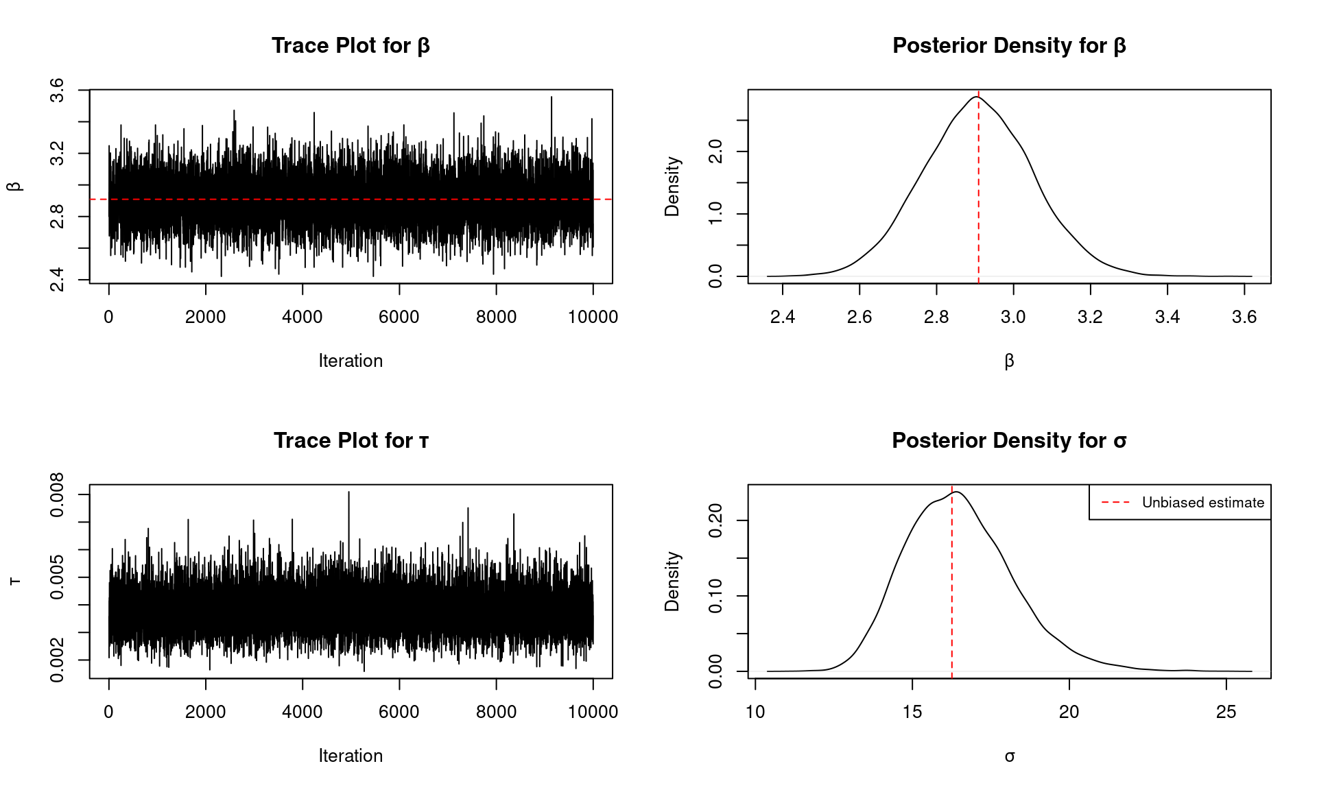

2.2.9.2 Summary Statistics

# Create summary table for Gibbs results
gibbs_summary <- data.frame(
  Parameter = rep(c("β", "σ"), each = 4),
  Statistic = rep(c("Mean", "Median", "SD", "95% CI"), 2),
  Value = c(
    round(mean(gibbs_results$beta), 4),
    round(median(gibbs_results$beta), 4),
    round(sd(gibbs_results$beta), 4),
    paste0("(", round(quantile(gibbs_results$beta, 0.025), 4), ", ", 
           round(quantile(gibbs_results$beta, 0.975), 4), ")"),
    round(mean(gibbs_results$sigma), 4),
    round(median(gibbs_results$sigma), 4),
    round(sd(gibbs_results$sigma), 4),
    paste0("(", round(quantile(gibbs_results$sigma, 0.025), 4), ", ", 
           round(quantile(gibbs_results$sigma, 0.975), 4), ")")
  )
)

kable(gibbs_summary, caption = "Posterior Summary from Gibbs Sampling", align = 'llr') %>%
  kable_styling(bootstrap_options = c("striped", "hover")) %>%
  pack_rows("β", 1, 4) %>%
  pack_rows("σ", 5, 8)

Posterior Summary from Gibbs Sampling

Parameter	Statistic	Value
β
β	Mean	2.9079
β	Median	2.9067
β	SD	0.1422
β	95% CI	(2.633, 3.1911)
σ
σ	Mean	16.4968
σ	Median	16.3794
σ	SD	1.7022
σ	95% CI	(13.5867, 20.2191)

# Comparison table
comparison_freq_bayes <- data.frame(
  Parameter = c("β", "σ"),
  `MLE (biased)` = c(round(beta_hat, 4), round(sigma_hat_mle, 4)),
  `MLE (unbiased)` = c(round(beta_hat, 4), round(sigma_hat_unbiased, 4)),
  `Posterior Mean` = c(round(mean(gibbs_results$beta), 4), round(mean(gibbs_results$sigma), 4)),
  check.names = FALSE
)

kable(comparison_freq_bayes, caption = "Comparison: Frequentist vs Bayesian Estimates", align = 'lrrr') %>%
  kable_styling(bootstrap_options = c("striped", "hover"))

Comparison: Frequentist vs Bayesian Estimates

Parameter	MLE (biased)	MLE (unbiased)	Posterior Mean
β	2.9091	2.9091	2.9079
σ	16.0958	16.2592	16.4968

2.2.10 Comparison with brms

# Fit model with brms (no intercept)
brms_model <- brm(dist ~ 0 + speed, 
                  data = cars,
                  prior = c(prior(normal(0, 31.62), class = "b"),  # SD = sqrt(1000)
                           prior(gamma(0.001, 0.001), class = "sigma")),
                  chains = 4, 
                  iter = 2000,
                  warmup = 1000,
                  seed = 123,
                  refresh = 0)

summary(brms_model)

 Family: gaussian 
  Links: mu = identity; sigma = identity 
Formula: dist ~ 0 + speed 
   Data: cars (Number of observations: 50) 
  Draws: 4 chains, each with iter = 2000; warmup = 1000; thin = 1;
         total post-warmup draws = 4000

Regression Coefficients:
      Estimate Est.Error l-95% CI u-95% CI Rhat Bulk_ESS Tail_ESS
speed     2.91      0.14     2.63     3.19 1.00     2908     2371

Further Distributional Parameters:
      Estimate Est.Error l-95% CI u-95% CI Rhat Bulk_ESS Tail_ESS
sigma    16.60      1.78    13.52    20.51 1.00     2981     2518

Draws were sampled using sampling(NUTS). For each parameter, Bulk_ESS
and Tail_ESS are effective sample size measures, and Rhat is the potential
scale reduction factor on split chains (at convergence, Rhat = 1).

# Create comparison table
comparison_gibbs_brms <- data.frame(
  Method = c("Manual Gibbs", "brms"),
  `β (Mean)` = c(round(mean(gibbs_results$beta), 4), round(fixef(brms_model)[1, 1], 4)),
  `β (SD)` = c(round(sd(gibbs_results$beta), 4), round(fixef(brms_model)[1, 2], 4)),
  check.names = FALSE
)

kable(comparison_gibbs_brms, caption = "Comparison: Manual Gibbs Sampling vs brms", align = 'lrr') %>%
  kable_styling(bootstrap_options = c("striped", "hover"))

Comparison: Manual Gibbs Sampling vs brms

Method	β (Mean)	β (SD)
Manual Gibbs	2.9079	0.1422
brms	2.9108	0.1448

2.2.11 3D Posterior Distribution

# Sample for visualization
sample_indices <- sample(length(gibbs_results$beta), 2000)
beta_sample <- gibbs_results$beta[sample_indices]
sigma_sample <- gibbs_results$sigma[sample_indices]

# Create density estimate
library(MASS)
dens <- kde2d(sigma_sample, beta_sample, n = 50)

plot_ly(x = dens$x, y = dens$y, z = dens$z) %>%
  add_surface() %>%
  add_markers(x = mean(sigma_sample), y = mean(beta_sample), z = max(dens$z),
              marker = list(size = 5, color = 'red'),
              name = 'Posterior Mean') %>%
  layout(scene = list(
    xaxis = list(title = 'σ'),
    yaxis = list(title = 'β'),
    zaxis = list(title = 'Posterior Density'),
    camera = list(eye = list(x = 1.5, y = 1.5, z = 1.3))
  ))

2.2.12 Joint Distribution Under Independent Priors

Under certain prior specifications that maintain independence between \(\beta\) and \(\tau\), we can derive closed-form marginal posteriors. Specifically, with independent priors where \(p(\beta, \tau) = p(\beta)p(\tau)\), we can integrate out one parameter to obtain marginal distributions.

Marginal for \(\beta\):

If we use an improper uniform prior for \(\beta\) and Jeffrey’s prior for \(\sigma^2\) (i.e., \(p(\beta, \sigma^2) \propto 1/\sigma^2\)), the marginal posterior for \(\beta\) follows a t-distribution:

\[\beta | \mathbf{y} \sim t_{n-1}\left(\hat{\beta}, \frac{\hat{\sigma}^2}{\sum x_i^2}\right)\]

where \(\hat{\beta} = \frac{\sum x_i y_i}{\sum x_i^2}\) and \(\hat{\sigma}^2 = \frac{\sum(y_i - \hat{\beta}x_i)^2}{n-1}\).

Marginal for \(\tau\):

With the same prior structure, after integrating out \(\beta\), the marginal posterior for \(\tau\) is:

\[\tau | \mathbf{y} \sim \text{Gamma}\left(\frac{n-1}{2}, \frac{RSS}{2}\right)\]

where \(RSS = \sum(y_i - \hat{\beta}x_i)^2\).

This special case provides closed-form posteriors but is limited to specific prior choices. The Gibbs sampling approach is more flexible and extends naturally to more complex models.

# Analytical t-distribution for beta
df <- length(y) - 1
scale <- sqrt(sigma_hat_unbiased^2 / sum(x^2))

# Create comparison table
comparison_analytical <- data.frame(
  Method = c("Analytical (t-dist)", "Gibbs Sampling"),
  Mean = c(round(beta_hat, 4), round(mean(gibbs_results$beta), 4)),
  SD = c(round(scale * sqrt(df/(df-2)), 4), round(sd(gibbs_results$beta), 4)),
  `95% CI Lower` = c(
    round(beta_hat + qt(0.025, df) * scale, 4),
    round(quantile(gibbs_results$beta, 0.025), 4)
  ),
  `95% CI Upper` = c(
    round(beta_hat + qt(0.975, df) * scale, 4),
    round(quantile(gibbs_results$beta, 0.975), 4)
  ),
  check.names = FALSE
)

kable(comparison_analytical, caption = "Comparison: Analytical vs Gibbs Sampling for β", align = 'lrrrr') %>%
  kable_styling(bootstrap_options = c("striped", "hover"))

Comparison: Analytical vs Gibbs Sampling for β

	Method	Mean	SD	95% CI Lower	95% CI Upper
	Analytical (t-dist)	2.9091	0.1443	2.625	3.1932
2.5%	Gibbs Sampling	2.9079	0.1422	2.633	3.1911

3 Logistic Regression

We now consider logistic regression for binary outcomes. The model is:

\[\log\left(\frac{P(Y_i = 1|X_i)}{1 - P(Y_i = 1|X_i)}\right) = \beta X_i\]

or equivalently:

\[P(Y_i = 1|X_i) = \frac{\exp(\beta X_i)}{1 + \exp(\beta X_i)} = \frac{1}{1 + \exp(-\beta X_i)}\]

Again, we omit the intercept for simplicity, though this is rarely done in practice.

3.1 Frequentist Estimation

3.1.1 Maximum Likelihood Estimation

The likelihood for logistic regression is based on the Bernoulli distribution:

\[L(\beta | \mathbf{y}, \mathbf{x}) = \prod_{i=1}^n p_i^{y_i}(1-p_i)^{1-y_i}\]

where \(p_i = \frac{1}{1 + \exp(-\beta x_i)}\).

The log-likelihood is:

\[\ell(\beta) = \sum_{i=1}^n \left[y_i \log(p_i) + (1-y_i)\log(1-p_i)\right]\]

\[= \sum_{i=1}^n \left[y_i \log\left(\frac{p_i}{1-p_i}\right) + \log(1-p_i)\right]\]

\[= \sum_{i=1}^n \left[y_i(\beta x_i) - \log(1 + \exp(\beta x_i))\right]\]

Deriving the MLE:

The score function (first derivative) is:

\[\frac{\partial \ell}{\partial \beta} = \sum_{i=1}^n \left[y_i x_i - \frac{x_i \exp(\beta x_i)}{1 + \exp(\beta x_i)}\right]\]

\[= \sum_{i=1}^n x_i(y_i - p_i) = 0\]

This equation does not have a closed-form solution and must be solved numerically using methods such as Newton-Raphson or iteratively reweighted least squares (IRLS).

Standard Error:

The observed information is:

\[\mathcal{I}(\beta) = -\frac{\partial^2 \ell}{\partial \beta^2} = \sum_{i=1}^n x_i^2 p_i(1-p_i)\]

The asymptotic variance of \(\hat{\beta}\) is:

\[\text{Var}(\hat{\beta}) = \frac{1}{\mathcal{I}(\hat{\beta})} = \frac{1}{\sum_{i=1}^n x_i^2 \hat{p}_i(1-\hat{p}_i)}\]

where \(\hat{p}_i = \frac{1}{1 + \exp(-\hat{\beta} x_i)}\).

3.1.2 Demonstration with Real Data

We’ll use a simple dataset to demonstrate logistic regression:

# Create a simple dataset
set.seed(456)
n <- 100
x_log <- rnorm(n, mean = 0, sd = 1)
true_beta <- 1.5
p_true <- 1 / (1 + exp(-true_beta * x_log))
y_log <- rbinom(n, 1, p_true)

# Store in dataframe
logistic_data <- data.frame(x = x_log, y = y_log)

# Manual maximum likelihood (using optim)
log_lik_logistic <- function(beta, y, x) {
  p <- 1 / (1 + exp(-beta * x))
  -sum(y * log(p) + (1 - y) * log(1 - p))
}

# Find MLE
mle_result <- optim(par = 0, fn = log_lik_logistic, y = y_log, x = x_log,
                    method = "BFGS", hessian = TRUE)

beta_hat_log <- mle_result$par
se_beta_log <- sqrt(solve(mle_result$hessian)[1,1])

# Verify with observed information
p_hat <- 1 / (1 + exp(-beta_hat_log * x_log))
obs_info <- sum(x_log^2 * p_hat * (1 - p_hat))
se_beta_formula <- sqrt(1 / obs_info)

# Create summary table
logistic_manual <- data.frame(
  Estimate = c("β̂", "SE(β̂) from optim", "SE(β̂) from formula"),
  Value = c(round(beta_hat_log, 4), round(se_beta_log, 4), round(se_beta_formula, 4))
)

kable(logistic_manual, caption = "Manual MLE for Logistic Regression", align = 'lr') %>%
  kable_styling(bootstrap_options = c("striped", "hover"))

Manual MLE for Logistic Regression

Estimate	Value
β̂	| 1.577
SE(β̂) from optim	| 0.334
SE(β̂) from formula	| 0.334

3.1.2.1 Comparison with glm()

# Fit with glm
logistic_glm <- glm(y ~ x - 1, data = logistic_data, family = binomial(link = "logit"))

# Create comparison table
comparison_glm <- data.frame(
  Estimate = c("β̂", "SE(β̂)"),
  Manual = c(round(beta_hat_log, 4), round(se_beta_log, 4)),
  `glm()` = c(round(coef(logistic_glm)[1], 4), round(summary(logistic_glm)$coefficients[1, 2], 4)),
  check.names = FALSE
)

kable(comparison_glm, caption = "Comparison: Manual MLE vs glm()", align = 'lrr') %>%
  kable_styling(bootstrap_options = c("striped", "hover"))

Comparison: Manual MLE vs glm()

	Estimate	Manual	glm()
x	β̂	| 1.577	| 1.577
	SE(β̂)	| 0.334	| 0.334

3.2 Bayesian Inference

For logistic regression, we don’t have conjugate priors in the traditional sense because the Bernoulli likelihood doesn’t combine nicely with standard distributions. However, we can use flexible approaches.

3.2.1 Metropolis-Hastings Algorithm

The Metropolis-Hastings (M-H) algorithm is a general MCMC method for sampling from distributions that don’t have a simple form. Unlike Gibbs sampling, which requires known conditional distributions, M-H can sample from any posterior distribution.

Basic Idea: M-H generates candidate values from a proposal distribution, then decides whether to accept or reject each candidate based on how well it fits the target posterior. This creates a Markov chain that eventually converges to samples from the posterior.

Algorithm Steps:

1. Start with an initial value \(\beta^{(0)}\)

2. For iteration \(t = 1, 2, \ldots, T\):

   • Propose a new value: \(\beta^* \sim q(\beta^* | \beta^{(t-1)})\) (proposal distribution)

   • Calculate acceptance ratio: \(r = \frac{p(\beta^* | \mathbf{y}) \cdot q(\beta^{(t-1)} | \beta^*)}{p(\beta^{(t-1)} | \mathbf{y}) \cdot q(\beta^* | \beta^{(t-1)})}\)

   • Accept $^* $ with probability \(\min(r, 1)\):

     • If accepted: \(\beta^{(t)} = \beta^*\)

     • If rejected: \(\beta^{(t)} = \beta^{(t-1)}\) (stay at current value)

The “random walk” proposal we use here is symmetric (\(q(\beta^* | \beta) = q(\beta | \beta^*)\)), so the proposal terms cancel and we only need the posterior ratio.

Important Notes:

• Proposal variance affects efficiency: too small = slow mixing, too large = low acceptance

• Target acceptance rate is typically 20-40% for complex models

• This goes beyond the scope of this course—see references for details

For more pedagogical introductions to M-H, see Chib & Greenberg (1995) and Robert & Casella (2011).

3.2.2 Gibbs Sampling with Data Augmentation

One approach is to place a normal prior on \(\beta\):

\[\beta \sim N(\mu_0, \sigma_0^2)\]

The posterior is:

\[p(\beta | \mathbf{y}) \propto p(\beta) \prod_{i=1}^n p_i^{y_i}(1-p_i)^{1-y_i}\]

This doesn’t have a closed form, so we use Metropolis-Hastings within Gibbs or other MCMC methods.

# Metropolis-Hastings sampler for logistic regression
mh_logistic <- function(y, x, n_iter = 10000, burn_in = 1000,
                        mu0 = 0, sigma0 = 10, proposal_sd = 0.1) {
  
  beta_samples <- numeric(n_iter)
  beta <- 0  # Initialize
  
  # Log posterior (unnormalized)
  log_posterior <- function(beta, y, x, mu0, sigma0) {
    p <- 1 / (1 + exp(-beta * x))
    log_lik <- sum(y * log(p) + (1 - y) * log(1 - p))
    log_prior <- dnorm(beta, mu0, sigma0, log = TRUE)
    log_lik + log_prior
  }
  
  accept_count <- 0
  
  for (i in 1:n_iter) {
    # Propose new beta
    beta_prop <- rnorm(1, beta, proposal_sd)
    
    # Calculate acceptance ratio
    log_ratio <- log_posterior(beta_prop, y, x, mu0, sigma0) -
                 log_posterior(beta, y, x, mu0, sigma0)
    
    # Accept/reject
    if (log(runif(1)) < log_ratio) {
      beta <- beta_prop
      if (i > burn_in) accept_count <- accept_count + 1
    }
    
    beta_samples[i] <- beta
  }
  
  cat("Acceptance rate:", accept_count / (n_iter - burn_in), "\n")
  
  list(beta = beta_samples[-(1:burn_in)])
}

# Run sampler
set.seed(789)
logistic_gibbs_results <- mh_logistic(y_log, x_log, n_iter = 11000, burn_in = 1000)

Acceptance rate: 0.9059 

3.2.2.1 Trace Plot and Summary

par(mfrow = c(1, 2))

plot(logistic_gibbs_results$beta, type = 'l', main = 'Trace Plot for β',
     xlab = 'Iteration', ylab = 'β')
abline(h = beta_hat_log, col = 'red', lty = 2)

plot(density(logistic_gibbs_results$beta), main = 'Posterior Density for β',
     xlab = 'β', ylab = 'Density', xlim = c(0, 3))
abline(v = beta_hat_log, col = 'red', lty = 2)
abline(v = true_beta, col = 'blue', lty = 2)
legend('topright', c('MLE', 'True β'), col = c('red', 'blue'), lty = 2)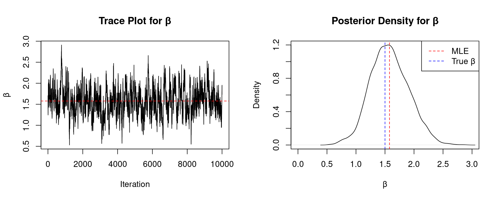

# Create summary table
logistic_gibbs_summary <- data.frame(
  Statistic = c("Mean", "Median", "SD", "95% CI"),
  Value = c(
    round(mean(logistic_gibbs_results$beta), 4),
    round(median(logistic_gibbs_results$beta), 4),
    round(sd(logistic_gibbs_results$beta), 4),
    paste0("(", round(quantile(logistic_gibbs_results$beta, 0.025), 4), ", ",
           round(quantile(logistic_gibbs_results$beta, 0.975), 4), ")")
  )
)

kable(logistic_gibbs_summary, caption = "Posterior Summary for β (Logistic Regression)", align = 'lr') %>%
  kable_styling(bootstrap_options = c("striped", "hover"))

Posterior Summary for β (Logistic Regression)

Statistic	Value
Mean	1.5792
Median	1.5648
SD	0.3307
95% CI	(0.9607, 2.2468)

# Comparison table
comparison_log_methods <- data.frame(
  Method = c("True β", "MLE", "Posterior Mean"),
  Value = c(round(true_beta, 4), round(beta_hat_log, 4), round(mean(logistic_gibbs_results$beta), 4))
)

kable(comparison_log_methods, caption = "Comparison: True vs Frequentist vs Bayesian", align = 'lr') %>%
  kable_styling(bootstrap_options = c("striped", "hover"))

Comparison: True vs Frequentist vs Bayesian

Method	Value
True β	1.5000
MLE	1.5773
Posterior Mean	1.5792

3.2.3 Comparison with brms

# Fit with brms
logistic_brms <- brm(y ~ 0 + x, 
                     data = logistic_data,
                     family = bernoulli(link = "logit"),
                     prior = prior(normal(0, 10), class = "b"),
                     chains = 4,
                     iter = 2000,
                     warmup = 1000,
                     seed = 789,
                     refresh = 0)

summary(logistic_brms)

 Family: bernoulli 
  Links: mu = logit 
Formula: y ~ 0 + x 
   Data: logistic_data (Number of observations: 100) 
  Draws: 4 chains, each with iter = 2000; warmup = 1000; thin = 1;
         total post-warmup draws = 4000

Regression Coefficients:
  Estimate Est.Error l-95% CI u-95% CI Rhat Bulk_ESS Tail_ESS
x     1.60      0.34     0.98     2.30 1.00     1403     1503

Draws were sampled using sampling(NUTS). For each parameter, Bulk_ESS
and Tail_ESS are effective sample size measures, and Rhat is the potential
scale reduction factor on split chains (at convergence, Rhat = 1).

# Create comparison table
comparison_log_gibbs_brms <- data.frame(
  Method = c("Manual M-H", "brms"),
  `β (Mean)` = c(round(mean(logistic_gibbs_results$beta), 4), round(fixef(logistic_brms)[1, 1], 4)),
  `β (SD)` = c(round(sd(logistic_gibbs_results$beta), 4), round(fixef(logistic_brms)[1, 2], 4)),
  check.names = FALSE
)

kable(comparison_log_gibbs_brms, caption = "Comparison: Manual Metropolis-Hastings vs brms", align = 'lrr') %>%
  kable_styling(bootstrap_options = c("striped", "hover"))

Comparison: Manual Metropolis-Hastings vs brms

Method	β (Mean)	β (SD)
Manual M-H	1.5792	0.3307
brms	1.5993	0.3416

3.2.4 Probit Regression via Auxiliary Variables

An alternative to logistic regression is probit regression, which uses the cumulative normal distribution:

\[P(Y_i = 1 | X_i) = \Phi(\beta X_i)\]

where \(\Phi\) is the standard normal CDF.

The auxiliary variable approach, developed by Albert & Chib (1993), introduces latent variables \(Z_i \sim N(\beta X_i, 1)\) where:

\[Y_i = \begin{cases} 1 & \text{if } Z_i > 0 \\ 0 & \text{if } Z_i \leq 0 \end{cases}\]

This formulation allows for straightforward Gibbs sampling:

1. Sample \(\beta | \mathbf{Z} \sim N(\mu_n, \sigma_n^2)\) (normal-normal conjugacy)

2. Sample \(Z_i | \beta, Y_i\) from truncated normal:

   • If \(Y_i = 1\): \(Z_i \sim N(\beta X_i, 1)\) truncated to \((0, \infty)\)

   • If \(Y_i = 0\): \(Z_i \sim N(\beta X_i, 1)\) truncated to \((-\infty, 0)\)

This method is particularly elegant because it converts a complex discrete outcome model into a straightforward continuous data model with truncation. The data augmentation strategy has been widely applied to other generalized linear models.

# Probit regression using auxiliary variables
library(truncnorm)

probit_gibbs <- function(y, x, n_iter = 10000, burn_in = 1000,
                         mu0 = 0, tau0 = 0.01) {
  
  n <- length(y)
  beta_samples <- numeric(n_iter)
  z <- rnorm(n)  # Initialize latent variables
  beta <- 0
  
  sum_x2 <- sum(x^2)
  
  for (i in 1:n_iter) {
    # Sample Z | beta, y
    mu_z <- beta * x
    for (j in 1:n) {
      if (y[j] == 1) {
        z[j] <- rtruncnorm(1, a = 0, b = Inf, mean = mu_z[j], sd = 1)
      } else {
        z[j] <- rtruncnorm(1, a = -Inf, b = 0, mean = mu_z[j], sd = 1)
      }
    }
    
    # Sample beta | Z (normal conjugate)
    tau_n <- sum_x2 + tau0
    mu_n <- (sum(x * z) + tau0 * mu0) / tau_n
    beta <- rnorm(1, mu_n, sqrt(1/tau_n))
    
    beta_samples[i] <- beta
  }
  
  list(beta = beta_samples[-(1:burn_in)])
}

# Run probit sampler
set.seed(789)
probit_results <- probit_gibbs(y_log, x_log, n_iter = 11000, burn_in = 1000)

# Create summary table
probit_summary <- data.frame(
  Statistic = c("Mean", "SD", "95% CI"),
  Value = c(
    round(mean(probit_results$beta), 4),
    round(sd(probit_results$beta), 4),
    paste0("(", round(quantile(probit_results$beta, 0.025), 4), ", ",
           round(quantile(probit_results$beta, 0.975), 4), ")")
  )
)

kable(probit_summary, caption = "Probit Posterior Summary for β", align = 'lr') %>%
  kable_styling(bootstrap_options = c("striped", "hover"))

Probit Posterior Summary for β

Statistic	Value
Mean	0.9312
SD	0.1832
95% CI	(0.5933, 1.3034)

# Note: Probit coefficients are on a different scale than logit
# Approximately: beta_logit ≈ 1.6 * beta_probit
comparison_scales <- data.frame(
  Model = c("Logit (MLE)", "Probit × 1.6"),
  `β estimate` = c(round(beta_hat_log, 4), round(mean(probit_results$beta) * 1.6, 4)),
  check.names = FALSE
)

kable(comparison_scales, caption = "Scale Comparison: Logit vs Probit (approximately)", align = 'lr') %>%
  kable_styling(bootstrap_options = c("striped", "hover"))

Scale Comparison: Logit vs Probit (approximately)

Model	β estimate
Logit (MLE)	1.5773
Probit × 1.6	1.4899

4 Summary

This document has presented foundational concepts in both Frequentist Estimation and Bayesian Inference approaches to regression modeling:

Linear Regression:

• Frequentist: Maximum likelihood and least squares produce identical point estimates

• Standard errors can be derived via Fisher information or variance principles

• Bayesian: Conditionally conjugate priors enable Gibbs sampling

• With appropriate priors, closed-form posteriors (t and gamma) are possible

Logistic Regression:

• Frequentist: Requires numerical optimization (no closed-form MLE)

• Bayesian: Metropolis-Hastings handles the non-conjugate posterior

• Probit alternative: Auxiliary variables enable efficient Gibbs sampling

These simplified models (no intercept) illustrate core principles that extend to more complex regression settings with multiple predictors, interactions, and hierarchical structures.

4.1 Why “Frequentist Estimation” vs “Bayesian Inference”?

The terminology distinction reflects fundamental philosophical and methodological differences:

Frequentist Estimation:

• View of parameters: Parameters are fixed, unknown constants

• Goal: Estimate the true parameter value from the data

• Uncertainty: Described through sampling distributions (e.g., “if we repeated this experiment many times and calculate many confidence intervals, 95% would contain the true parameter”)

• Output: Point estimates with standard errors and confidence intervals

• Interpretation: “We estimate β = 2.7 with 95% CI (2.1, 3.3)” means the procedure would capture the true value 95% of the time across repeated samples

Bayesian Inference:

• View of parameters: Parameters are random variables with probability distributions

• Goal: Update our beliefs about parameters using data (prior → posterior)

• Uncertainty: Described through probability distributions directly on parameters

• Output: Full posterior distributions, summarized with credible intervals

• Interpretation: “P(2.1 < β < 3.3 | data) = 0.95” means there’s a 95% probability that β lies in this interval given the observed data

The distinction matters because:

• Bayesians don’t “estimate” a fixed value—they make probabilistic statements about parameters

• The interpretation of uncertainty differs fundamentally between approaches

• Each framework has its own logic for inference, prediction, and decision-making

Understanding both perspectives enriches your statistical toolkit and helps you communicate appropriately with different audiences.

5 References

Bayesian Inference and MCMC:

Albert, J. H., & Chib, S. (1993). Bayesian analysis of binary and polychotomous response data. Journal of the American Statistical Association, 88(422), 669-679.

Chib, S., & Greenberg, E. (1995). Understanding the Metropolis-Hastings algorithm. The American Statistician, 49(4), 327-335.

Gelman, A., Carlin, J. B., Stern, H. S., Dunson, D. B., Vehtari, A., & Rubin, D. B. (2013). Bayesian Data Analysis (3rd ed.). Chapman and Hall/CRC.

Robert, C. P., & Casella, G. (2011). A short history of Markov Chain Monte Carlo: Subjective recollections from incomplete data. Statistical Science, 26(1), 102-115.

Software:

Bürkner, P. C. (2017). brms: An R package for Bayesian multilevel models using Stan. Journal of Statistical Software, 80(1), 1-28.

Note: A full course on Bayesian regression methods would allow deeper exploration of these topics, including more complex models, prior specification strategies, model comparison, and advanced MCMC diagnostics. The material presented here serves as an introduction.