Multiple Imputation in R

Chris Slaughter

April 13, 2026

Code

library(mice)
library(naniar)
library(VIM)
library(sandwich)
library(lmtest)
library(ggplot2)
library(knitr)
library(kableExtra)

1 Introduction

These notes supplement the primary lecture notes on missing data (Set13.pdf), which cover the conceptual foundations of missing data mechanisms (MCAR, MAR, MNAR), the limitations of ad hoc methods, inverse probability weighting, and multiple imputation. The purpose of these supplementary notes is to:

Provide a synthetic dataset that illustrates common missingness patterns encountered in clinical research
Demonstrate the consequences of ad hoc missing data methods through direct comparison
Implement inverse probability weighting as a principled alternative
Walk through multiple imputation using the mice package, including diagnostics and convergence assessment
Introduce the Hmisc/rms approach to multiple imputation
Discuss practical considerations for applied work

2 Setup and Data

2.1 A Synthetic Clinical Trial Dataset

We construct a synthetic dataset loosely modeled on a randomized trial of a blood pressure medication
The dataset contains 500 subjects with:
- treatment: Randomized treatment assignment (0 = placebo, 1 = active)
- age: Age in years (continuous)
- sex: Sex (0 = male, 1 = female)
- bmi: Body mass index at baseline (continuous)
- sbp_base: Systolic blood pressure at baseline (continuous)
- sbp_6mo: Systolic blood pressure at 6 months (continuous, the primary outcome)
- side_effects: Whether the subject reported side effects (binary)
Missingness is introduced in sbp_6mo and bmi with different mechanisms:
- sbp_6mo is more likely to be missing when subjects have higher baseline SBP and are on active treatment (simulating dropout due to side effects or perceived lack of efficacy). This is MAR
- bmi is missing completely at random in a small fraction of subjects. This is MCAR

Code

set.seed(2024)
n <- 500

## Generate complete data
treatment   <- rbinom(n, 1, 0.5)
age         <- round(rnorm(n, mean = 55, sd = 10), 1)
sex         <- rbinom(n, 1, 0.45)
bmi         <- round(rnorm(n, mean = 28, sd = 5), 1)
sbp_base    <- round(rnorm(n, mean = 145, sd = 15), 0)
side_effects <- rbinom(n, 1, plogis(-2 + 0.8 * treatment + 0.01 * sbp_base))

## True treatment effect: -8 mmHg reduction in SBP at 6 months
sbp_6mo <- round(sbp_base - 8 * treatment + 0.3 * (age - 55) +
                   0.4 * (bmi - 28) + rnorm(n, 0, 10), 0)

dat_complete <- data.frame(treatment, age, sex, bmi, sbp_base,
                           side_effects, sbp_6mo)

## Introduce MAR missingness in sbp_6mo
## Higher baseline SBP and active treatment increase probability of dropout
prob_miss_sbp <- plogis(-3 + 0.015 * sbp_base + 0.6 * treatment +
                          0.5 * side_effects)
miss_sbp <- rbinom(n, 1, prob_miss_sbp)

## Introduce MCAR missingness in bmi (10% completely at random)
miss_bmi <- rbinom(n, 1, 0.10)

## Create the analysis dataset with missing values
dat <- dat_complete
dat$sbp_6mo[miss_sbp == 1] <- NA
dat$bmi[miss_bmi == 1]     <- NA

summary(dat)

   treatment          age             sex             bmi          sbp_base    
 Min.   :0.000   Min.   :29.20   Min.   :0.000   Min.   :15.7   Min.   :101.0  
 1st Qu.:0.000   1st Qu.:48.50   1st Qu.:0.000   1st Qu.:24.9   1st Qu.:135.0  
 Median :1.000   Median :54.50   Median :0.000   Median :27.7   Median :146.0  
 Mean   :0.516   Mean   :54.99   Mean   :0.454   Mean   :28.1   Mean   :145.2  
 3rd Qu.:1.000   3rd Qu.:62.02   3rd Qu.:1.000   3rd Qu.:31.2   3rd Qu.:155.2  
 Max.   :1.000   Max.   :84.30   Max.   :1.000   Max.   :40.7   Max.   :186.0  
                                                 NA's   :47                    
  side_effects      sbp_6mo     
 Min.   :0.000   Min.   : 89.0  
 1st Qu.:0.000   1st Qu.:131.0  
 Median :0.000   Median :140.5  
 Mean   :0.488   Mean   :141.8  
 3rd Qu.:1.000   3rd Qu.:154.0  
 Max.   :1.000   Max.   :190.0  
                 NA's   :228

We retain dat_complete so we can compare methods against the “truth” later
In practice, we never have dat_complete. This is the advantage of a simulation exercise

Code

## Missingness rates
colMeans(is.na(dat)) |> round(3)

   treatment          age          sex          bmi     sbp_base side_effects 
       0.000        0.000        0.000        0.094        0.000        0.000 
     sbp_6mo 
       0.456

3 Exploring and Characterizing Missingness

Before choosing a method for handling missing data, we must understand the pattern and potential mechanism of missingness
Key questions:
- Which variables are missing and how much?
- Do the missing values co-occur?
- Do the observed characteristics of subjects with and without missing data differ?
- Is there evidence against MCAR?

3.1 Missing Data Patterns

Code

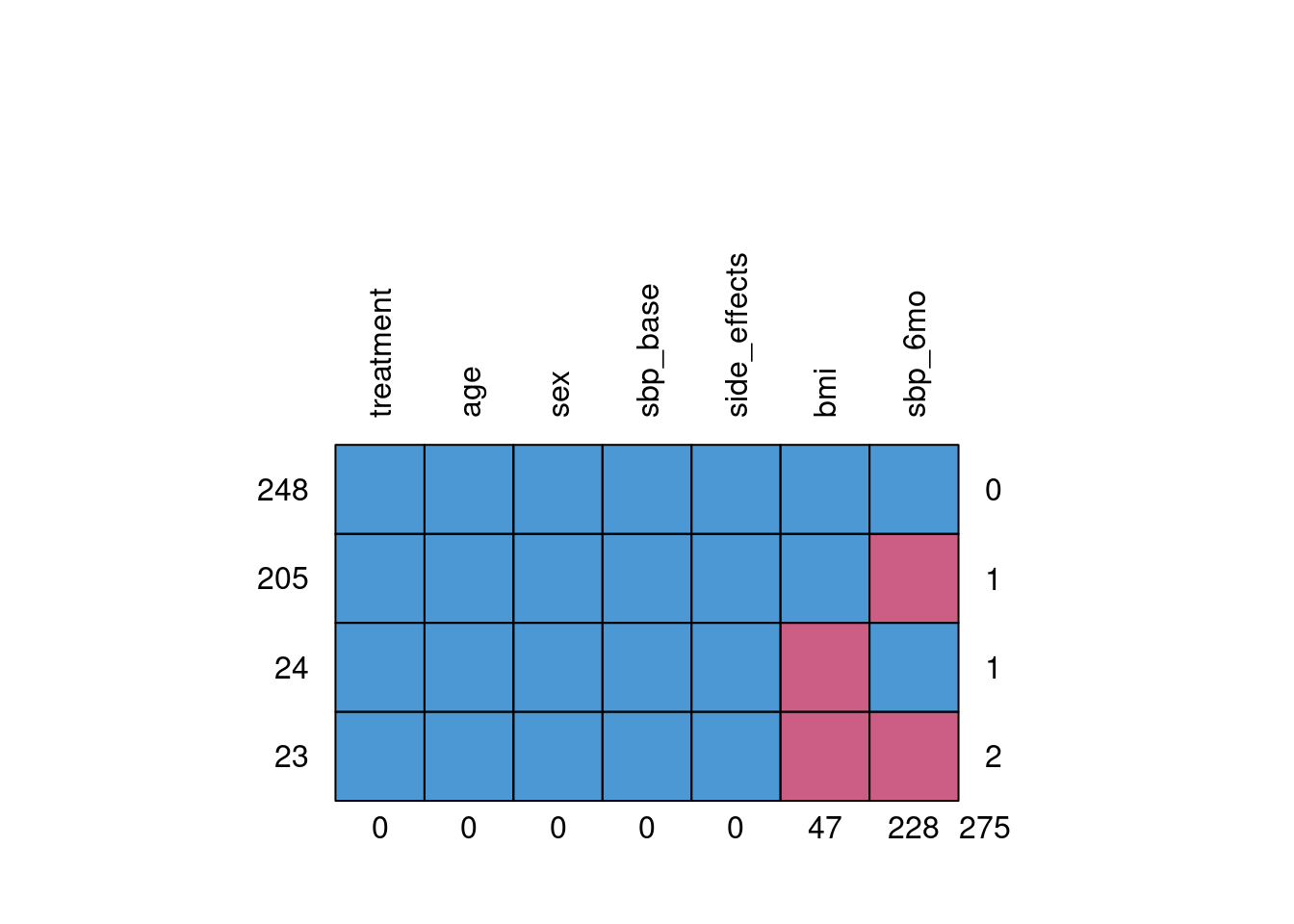
md.pattern(dat, rotate.names = TRUE)

    treatment age sex sbp_base side_effects bmi sbp_6mo    
248         1   1   1        1            1   1       1   0
205         1   1   1        1            1   1       0   1
24          1   1   1        1            1   0       1   1
23          1   1   1        1            1   0       0   2
            0   0   0        0            0  47     228 275

Each row is a unique pattern of observed (1) and missing (0) values
The left margin counts the number of observations with each pattern
The bottom margin counts the total number of missing values per variable

3.2 Visualizing Missingness

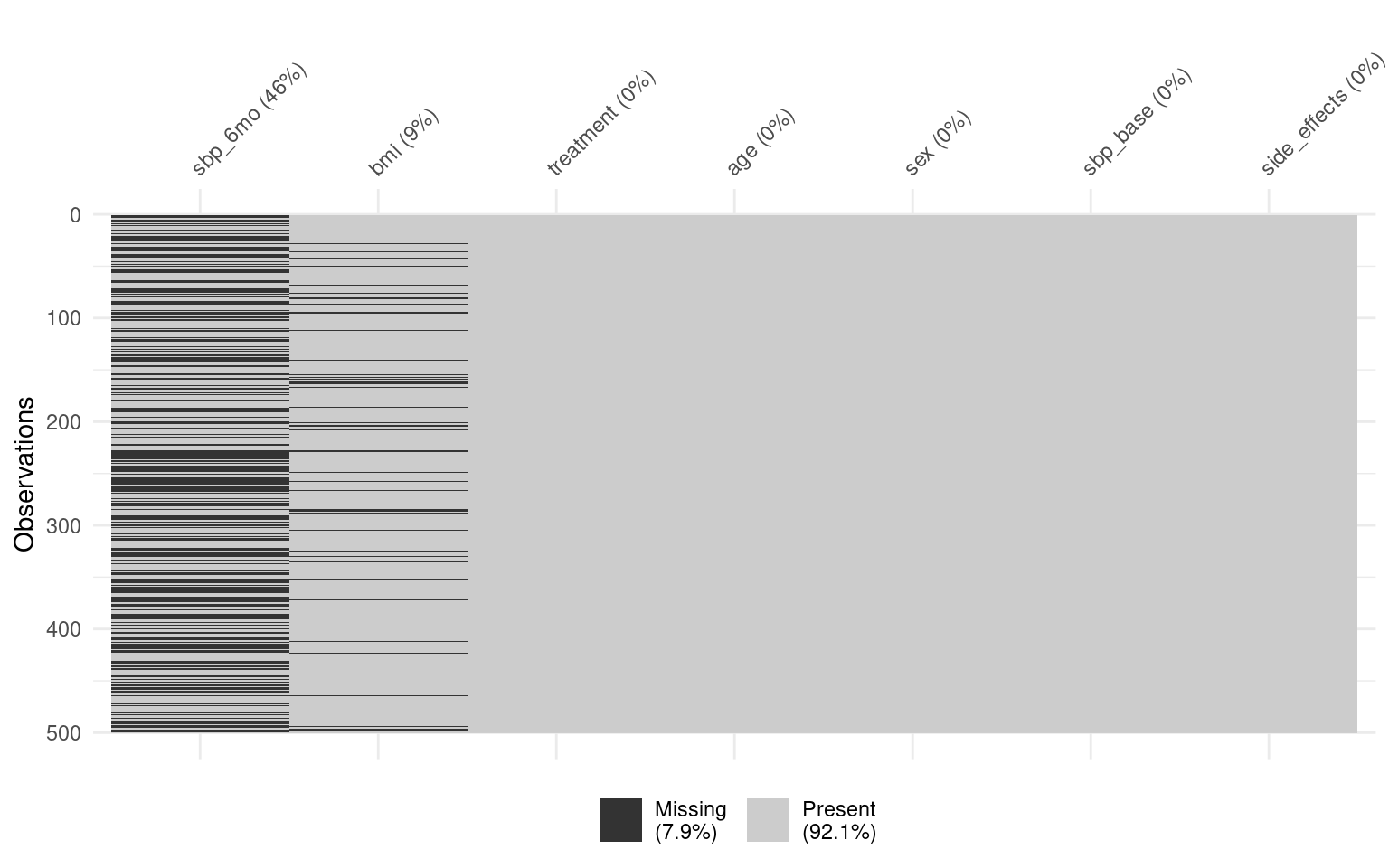
vis_miss() provides a heatmap of the full dataset, showing where missing values occur

Code

vis_miss(dat, sort_miss = TRUE)

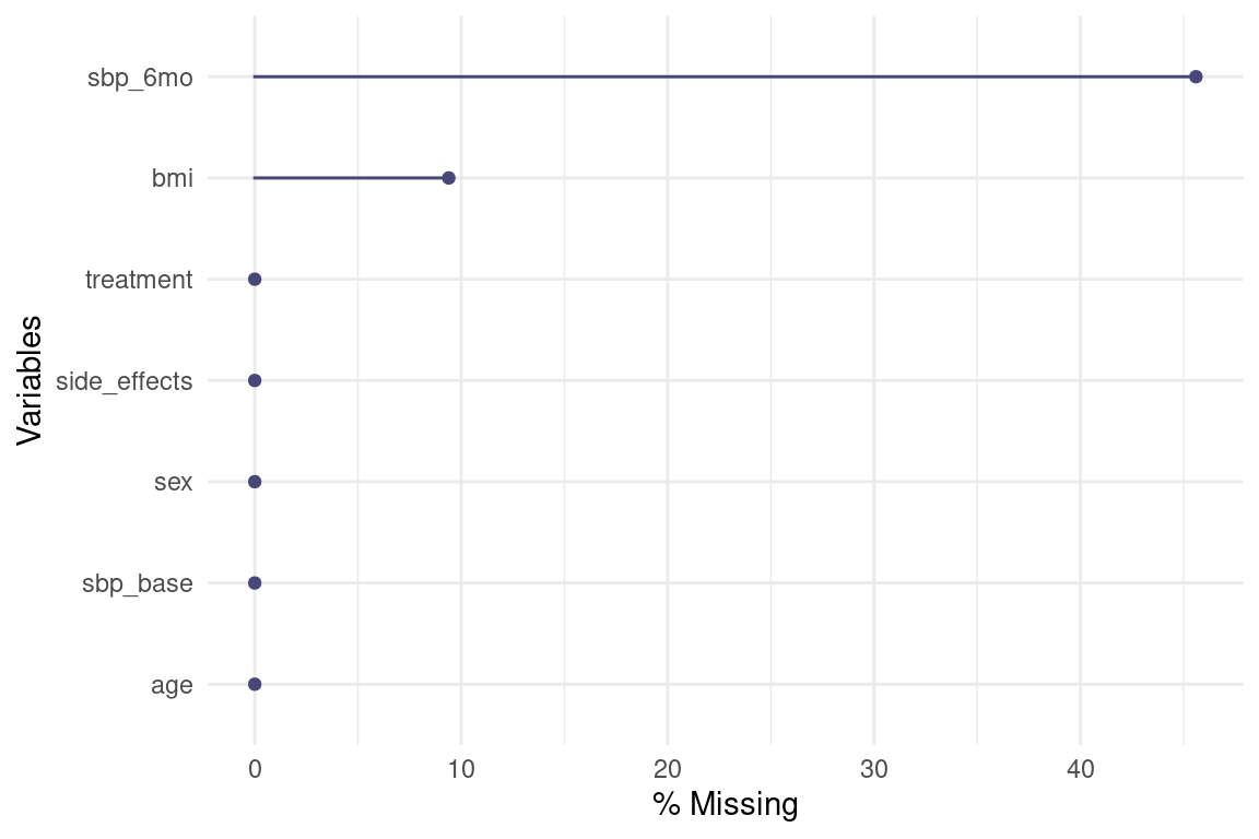
gg_miss_var() shows the number and percentage of missing values per variable

Code

gg_miss_var(dat, show_pct = TRUE)

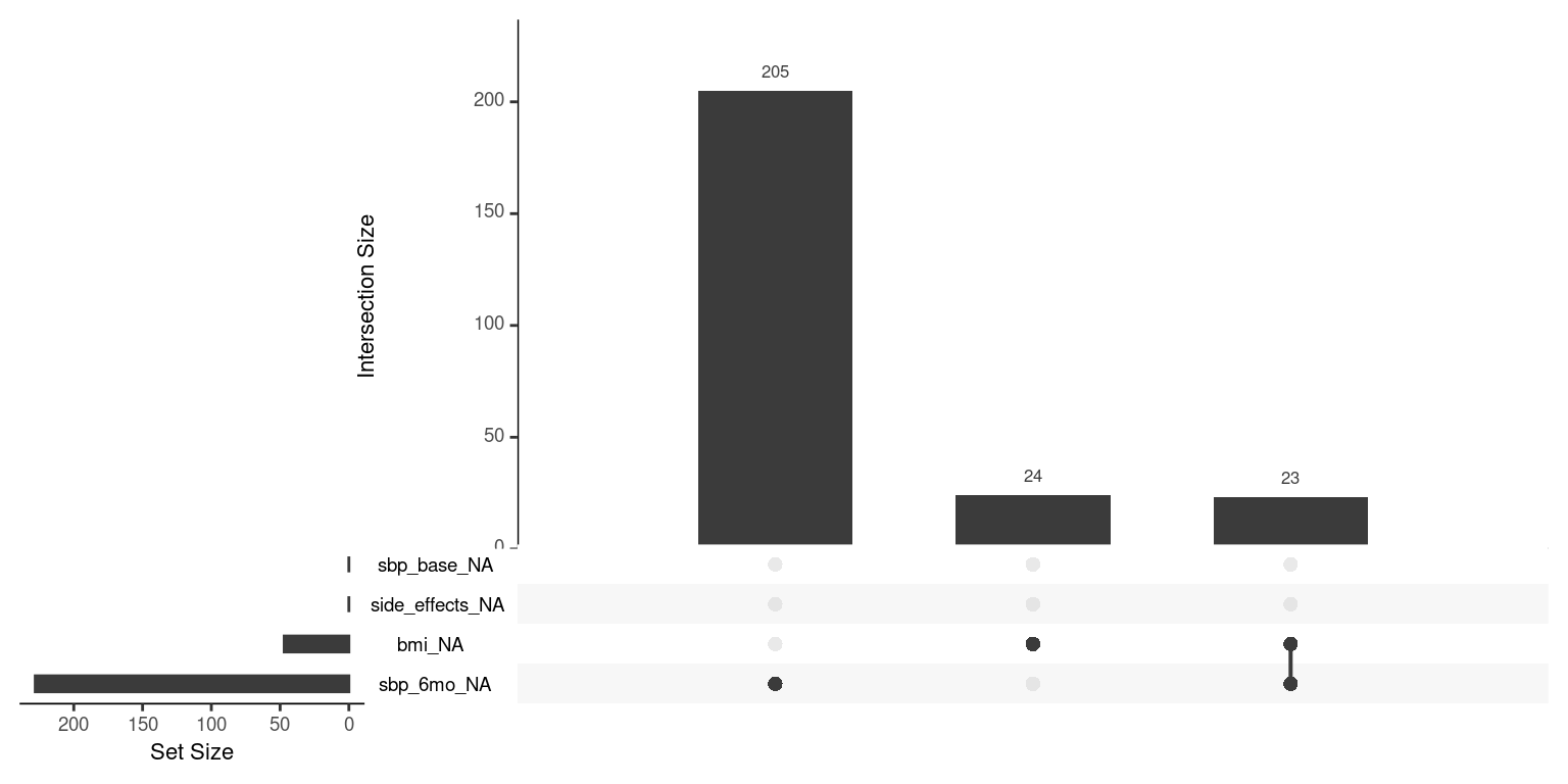
gg_miss_upset() displays the intersection of missingness across variables
- Useful for understanding whether missingness in different variables tends to co-occur

Code

gg_miss_upset(dat)

3.3 Comparing Observed Characteristics by Missingness Status

If subjects with missing sbp_6mo differ systematically from those with observed sbp_6mo, the data are likely not MCAR
We can examine this by comparing baseline characteristics across missingness groups

Code

dat$miss_sbp <- factor(is.na(dat$sbp_6mo),
                       levels = c(FALSE, TRUE),
                       labels = c("Observed", "Missing"))

## Compare baseline characteristics
aggregate(cbind(age, sbp_base, side_effects) ~ miss_sbp + treatment,
          data = dat, FUN = mean) |>
  kable(digits = 2) |>
  kable_styling(bootstrap_options = "striped", full_width = FALSE)

miss_sbp	treatment	age	sbp_base	side_effects
Observed	0	55.59	144.07	0.34
Missing	0	56.29	147.32	0.46
Observed	1	54.41	144.47	0.49
Missing	1	54.05	145.74	0.66

If baseline SBP or treatment assignment differs between observed and missing groups, this is evidence against MCAR (but consistent with MAR)

3.4 Little’s MCAR Test

Little’s test is a formal test of the MCAR assumption
- \(H_0\): The data are MCAR
- \(H_1\): The data are not MCAR
Rejection of \(H_0\) suggests the data are not MCAR, but does not distinguish between MAR and MNAR

Code

mcar_test(dat[, c("age", "sex", "bmi", "sbp_base",
                   "treatment", "side_effects", "sbp_6mo")])

# A tibble: 1 × 4
  statistic    df   p.value missing.patterns
      <dbl> <dbl>     <dbl>            <int>
1      51.9    17 0.0000215                4

A small \(p\)-value provides evidence against MCAR
Note that failure to reject does not confirm MCAR. The test has limited power, especially with small samples or few missing data patterns

3.5 Margin Plots

VIM::marginplot() provides a bivariate view of missingness
- The main panel shows the scatterplot for complete cases
- The margins show the distribution of each variable when the other is missing

Code

marginplot(dat[, c("sbp_base", "sbp_6mo")],
           col  = c("blue", "red", "orange"),
           pch  = 20)

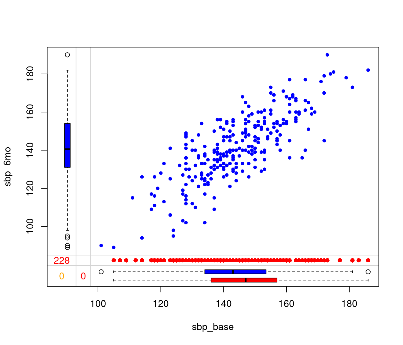
If the marginal distributions (red) differ from the complete cases (blue), this suggests the missingness in one variable is related to the values of the other

Code

## Remove the missingness indicator (not needed for analysis)
dat$miss_sbp <- NULL

4 Ad Hoc Methods: A Demonstration

The primary notes describe several ad hoc approaches to handling missing data and their limitations
Here we implement the most common ones on our synthetic data and compare the results to the truth (the complete data analysis)
This makes the theoretical critique concrete

4.1 The True Treatment Effect

Because we simulated the data, we know the true treatment effect and can compute the “gold standard” analysis on the complete data

Code

## Analysis on the full (no missingness) data
fit_true <- lm(sbp_6mo ~ treatment + age + sex + bmi + sbp_base, data = dat_complete)
coef(summary(fit_true))["treatment", ] |> round(4)

  Estimate Std. Error    t value   Pr(>|t|) 
   -8.2757     0.8779    -9.4266     0.0000

4.2 Complete Case Analysis

Discard all observations with any missing values and analyze only the complete cases
This is the default behavior of most R modeling functions

Code

fit_cc <- lm(sbp_6mo ~ treatment + age + sex + bmi + sbp_base, data = dat)
coef(summary(fit_cc))["treatment", ] |> round(4)

  Estimate Std. Error    t value   Pr(>|t|) 
   -8.5101     1.3115    -6.4890     0.0000

Compare the treatment effect estimate to the truth
Note also the change in sample size:

Code

nobs(fit_cc)

[1] 248

Complete case analysis:
- Reduces sample size and precision
- Can be biased when data are not MCAR
- In our example, dropout depends on treatment and baseline SBP, so MCAR does not hold and the treatment effect estimate may be biased

4.3 Last Observation Carried Forward (LOCF)

LOCF assumes that the missing 6-month SBP equals the baseline SBP
- This is a strong and often implausible assumption
- It implies no change over time for subjects with missing data

Code

dat_locf <- dat
dat_locf$sbp_6mo[is.na(dat_locf$sbp_6mo)] <-
  dat_locf$sbp_base[is.na(dat_locf$sbp_6mo)]

fit_locf <- lm(sbp_6mo ~ treatment + age + sex + bmi + sbp_base, data = dat_locf)
coef(summary(fit_locf))["treatment", ] |> round(4)

  Estimate Std. Error    t value   Pr(>|t|) 
   -3.8665     0.7536    -5.1309     0.0000

LOCF typically attenuates the treatment effect because it assumes dropouts experienced no benefit (or harm) from treatment
The standard errors do not account for the fact that many “observed” values are actually carried forward. They are too small, giving a false sense of precision

4.4 Mean Imputation

Replace missing sbp_6mo with the overall mean of the observed values
This preserves the sample mean but distorts the variance, correlations, and regression relationships

Code

dat_mean <- dat
dat_mean$sbp_6mo[is.na(dat_mean$sbp_6mo)] <- mean(dat$sbp_6mo, na.rm = TRUE)

fit_mean <- lm(sbp_6mo ~ treatment + age + sex + bmi + sbp_base, data = dat_mean)
coef(summary(fit_mean))["treatment", ] |> round(4)

  Estimate Std. Error    t value   Pr(>|t|) 
   -4.2115     1.0216    -4.1225     0.0000

Mean imputation:
- Biases regression coefficients toward zero (attenuates associations)
- Underestimates variance because imputed values have no variability
- Produces artificially narrow confidence intervals

4.5 Comparison of Ad Hoc Methods

Code

results <- data.frame(
  Method    = c("Truth (complete data)", "Complete case",
                "LOCF", "Mean imputation"),
  Estimate  = c(coef(fit_true)["treatment"],
                coef(fit_cc)["treatment"],
                coef(fit_locf)["treatment"],
                coef(fit_mean)["treatment"]),
  SE        = c(coef(summary(fit_true))["treatment", "Std. Error"],
                coef(summary(fit_cc))["treatment", "Std. Error"],
                coef(summary(fit_locf))["treatment", "Std. Error"],
                coef(summary(fit_mean))["treatment", "Std. Error"]),
  N         = c(nobs(fit_true), nobs(fit_cc), nobs(fit_locf), nobs(fit_mean))
)

results |>
  kable(digits = 4, row.names = FALSE) |>
  kable_styling(bootstrap_options = "striped", full_width = FALSE)

Method	Estimate	SE	N
Truth (complete data)	-8.2757	0.8779	500
Complete case	-8.5101	1.3115	248
LOCF	-3.8665	0.7536	453
Mean imputation	-4.2115	1.0216	453

The degree of bias and efficiency loss varies by method, but all ad hoc approaches share a common weakness: they do not properly account for the uncertainty introduced by missing data

5 Inverse Probability Weighting

5.1 Overview

Inverse probability weighting (IPW) is a principled approach for handling MAR data
The idea:
- Estimate the probability that each observation is observed (i.e., not missing) given the observed covariates
- Weight each observed subject by the inverse of their observation probability
- Subjects who are observed but “similar to” subjects who dropped out receive higher weights, compensating for the missing data
IPW requires a missingness model, typically a logistic regression predicting the probability of being observed

5.2 Implementation

Step 1: Fit a logistic regression model for the probability of observing sbp_6mo

Code

## Missingness model: predict P(observed)
miss_model <- glm(is.na(sbp_6mo) ~ treatment + age + sex + sbp_base + side_effects,
                  data = dat, family = binomial)
summary(miss_model)


Call:
glm(formula = is.na(sbp_6mo) ~ treatment + age + sex + sbp_base + 
    side_effects, family = binomial, data = dat)

Coefficients:
              Estimate Std. Error z value Pr(>|z|)    
(Intercept)  -2.817354   1.159375  -2.430 0.015096 *  
treatment     0.838086   0.190305   4.404 1.06e-05 ***
age           0.003297   0.009805   0.336 0.736660    
sex          -0.035836   0.188261  -0.190 0.849033    
sbp_base      0.011854   0.006411   1.849 0.064471 .  
side_effects  0.629307   0.189746   3.317 0.000911 ***
---
Signif. codes:  0 '***' 0.001 '**' 0.01 '*' 0.05 '.' 0.1 ' ' 1

(Dispersion parameter for binomial family taken to be 1)

    Null deviance: 689.27  on 499  degrees of freedom
Residual deviance: 649.27  on 494  degrees of freedom
AIC: 661.27

Number of Fisher Scoring iterations: 4

Code

## Predicted probability of being observed
p_obs <- 1 - predict(miss_model, type = "response")

## Inverse probability weights (only for observed subjects)
dat$ipw <- ifelse(!is.na(dat$sbp_6mo), 1 / p_obs, NA)

## Examine the distribution of weights
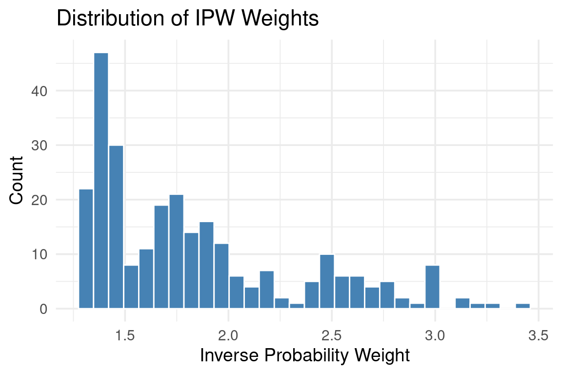
summary(dat$ipw[!is.na(dat$sbp_6mo)])

   Min. 1st Qu.  Median    Mean 3rd Qu.    Max. 
  1.279   1.417   1.710   1.837   2.044   3.391

Very large weights indicate subjects who were unlikely to be observed but were. These can make IPW estimates unstable
A common diagnostic is to check whether any weights are extremely large relative to the rest

Code

ggplot(dat[!is.na(dat$sbp_6mo), ], aes(x = ipw)) +
  geom_histogram(bins = 30, fill = "steelblue", color = "white") +
  labs(x = "Inverse Probability Weight", y = "Count",
       title = "Distribution of IPW Weights") +
  theme_minimal(base_size = 14)

Step 2: Fit the analysis model using the IPW weights

Code

fit_ipw <- lm(sbp_6mo ~ treatment + age + sex + bmi + sbp_base,
              data = dat, weights = ipw)
coef(summary(fit_ipw))["treatment", ] |> round(4)

  Estimate Std. Error    t value   Pr(>|t|) 
   -8.1456     1.3107    -6.2149     0.0000

The standard errors from a weighted lm() are not fully correct for IPW. They do not account for the estimation of the weights
Two approaches to obtaining more appropriate standard errors:
- Robust (sandwich) standard errors via the sandwich package
- Bootstrap standard errors that re-estimate both the weights and the analysis model in each replicate

5.2.1 Sandwich Standard Errors

The sandwich (Huber-White) estimator provides heteroscedasticity-consistent standard errors
In the IPW context, this accounts for the heterogeneous variance introduced by weighting but does not fully account for uncertainty in the weight estimation step
- It is an improvement over the naive model-based SE, but still an approximation

Code

## Robust (HC1) standard errors
ipw_robust <- coeftest(fit_ipw, vcov = vcovHC(fit_ipw, type = "HC1"))
ipw_robust["treatment", ] |> round(4)

  Estimate Std. Error    t value   Pr(>|t|) 
   -8.1456     1.3745    -5.9263     0.0000

5.2.2 Bootstrap Standard Errors

The bootstrap re-estimates the entire IPW procedure (missingness model \(\rightarrow\) weights \(\rightarrow\) analysis model) on each resampled dataset
This correctly propagates the uncertainty from the weight estimation step into the standard errors

Code

set.seed(12345)
n_boot <- 1000

boot_ests <- numeric(n_boot)
for (b in seq_len(n_boot)) {
  ## Resample with replacement
  idx <- sample(seq_len(nrow(dat)), replace = TRUE)
  dat_b <- dat[idx, ]

  ## Re-estimate the missingness model
  miss_b <- glm(is.na(sbp_6mo) ~ treatment + age + sex + sbp_base + side_effects,
                data = dat_b, family = binomial)
  p_obs_b <- 1 - predict(miss_b, type = "response")

  ## Compute weights (observed subjects only)
  dat_b$ipw_b <- ifelse(!is.na(dat_b$sbp_6mo), 1 / p_obs_b, NA)

  ## Fit the weighted analysis model
  fit_b <- lm(sbp_6mo ~ treatment + age + sex + bmi + sbp_base,
              data = dat_b, weights = ipw_b)
  boot_ests[b] <- coef(fit_b)["treatment"]
}

## Bootstrap SE is the standard deviation of the bootstrap estimates
se_boot <- sd(boot_ests)
se_boot |> round(4)

[1] 1.3349

5.2.3 Comparing IPW Standard Errors

Code

data.frame(
  SE_Method = c("Naive (model-based)", "Sandwich (HC1)", "Bootstrap"),
  SE        = c(coef(summary(fit_ipw))["treatment", "Std. Error"],
                ipw_robust["treatment", "Std. Error"],
                se_boot)
) |>
  kable(digits = 4, row.names = FALSE) |>
  kable_styling(bootstrap_options = "striped", full_width = FALSE)

SE_Method	SE
Naive (model-based)	1.3107
Sandwich (HC1)	1.3745
Bootstrap	1.3349

The naive SE ignores both the heterogeneous weighting and the uncertainty in weight estimation
The sandwich SE corrects for heterogeneous variance but not for estimated weights
The bootstrap SE accounts for both sources of uncertainty and is generally preferred

5.3 Limitations of IPW

IPW uses only the observed data. It does not fill in missing values
If the missingness model is misspecified, the weights will be wrong and the estimates biased
Extreme weights can make estimates unstable
- Weight trimming or stabilized weights can help but introduce a different form of bias
IPW is most useful when the outcome is missing but covariates are complete
- When covariates are also missing, the approach becomes more complex

Code

## Remove the IPW column (not needed for subsequent analyses)
dat$ipw <- NULL

6 Multiple Imputation with `mice`

6.1 The MICE Algorithm

Multiple Imputation by Chained Equations (MICE) is the most widely used MI framework
The algorithm:
1. Initialize missing values with simple imputations (e.g., random draws from observed values)
2. For each variable with missing data, fit a regression model using all other variables as predictors and draw imputed values from the posterior predictive distribution
3. Cycle through all variables with missing data. One complete cycle is one iteration
4. Repeat for several iterations until the distributions stabilize (convergence)
5. The result is one imputed dataset; repeat the entire process \(m\) times to get \(m\) imputed datasets
Each imputed dataset is analyzed separately, and the results are combined using Rubin’s rules

6.2 Running `mice()`

Code

imp <- mice(dat, m = 20, maxit = 10, seed = 12345, print = FALSE)
imp

Class: mids
Number of multiple imputations:  20 
Imputation methods:
   treatment          age          sex          bmi     sbp_base side_effects 
          ""           ""           ""        "pmm"           ""           "" 
     sbp_6mo 
       "pmm" 
PredictorMatrix:
             treatment age sex bmi sbp_base side_effects sbp_6mo
treatment            0   1   1   1        1            1       1
age                  1   0   1   1        1            1       1
sex                  1   1   0   1        1            1       1
bmi                  1   1   1   0        1            1       1
sbp_base             1   1   1   1        0            1       1
side_effects         1   1   1   1        1            0       1

m = 20: Create 20 imputed datasets
- Modern guidance suggests \(m\) should be at least as large as the percentage of incomplete cases
maxit = 10: Run 10 iterations per imputation
print = FALSE: Suppress iteration-by-iteration output

6.3 The Methods Vector

The method vector specifies the imputation model for each variable
mice chooses defaults based on variable type:
- Continuous: "pmm" (predictive mean matching)
- Binary: "logreg" (logistic regression)
- Unordered categorical: "polyreg" (polytomous logistic regression)
- Ordered categorical: "polr" (proportional odds model)
Variables with no missing data have "" (empty string). They are not imputed but are used as predictors

Code

imp$method

   treatment          age          sex          bmi     sbp_base side_effects 
          ""           ""           ""        "pmm"           ""           "" 
     sbp_6mo 
       "pmm"

Predictive mean matching (PMM) is the default for continuous variables
- PMM draws imputed values from the observed data, so imputations are always within the range of observed values
- This is more robust to model misspecification than Bayesian linear regression ("norm")
To change a method:

Code

## Example: switch bmi to Bayesian linear regression
meth <- imp$method
meth["bmi"] <- "norm"
meth

   treatment          age          sex          bmi     sbp_base side_effects 
          ""           ""           ""       "norm"           ""           "" 
     sbp_6mo 
       "pmm"

6.4 The Predictor Matrix

The predictor matrix controls which variables are used to impute which
- Rows = variable being imputed; Columns = predictors
- 1 = included as predictor; 0 = excluded
- Diagonal is always 0 (a variable does not predict itself)

Code

imp$predictorMatrix

             treatment age sex bmi sbp_base side_effects sbp_6mo
treatment            0   1   1   1        1            1       1
age                  1   0   1   1        1            1       1
sex                  1   1   0   1        1            1       1
bmi                  1   1   1   0        1            1       1
sbp_base             1   1   1   1        0            1       1
side_effects         1   1   1   1        1            0       1
sbp_6mo              1   1   1   1        1            1       0

By default, every other variable is used as a predictor for each imputed variable
To modify (e.g., exclude side_effects from the imputation model for bmi):

Code

pred <- imp$predictorMatrix
pred["bmi", "side_effects"] <- 0
pred

             treatment age sex bmi sbp_base side_effects sbp_6mo
treatment            0   1   1   1        1            1       1
age                  1   0   1   1        1            1       1
sex                  1   1   0   1        1            1       1
bmi                  1   1   1   0        1            0       1
sbp_base             1   1   1   1        0            1       1
side_effects         1   1   1   1        1            0       1
sbp_6mo              1   1   1   1        1            1       0

An important practical point: the outcome (sbp_6mo) should be included as a predictor in the imputation model for covariates like bmi, even though sbp_6mo is not missing in those observations
- Omitting the outcome from the imputation model biases the imputed covariate values and attenuates the association between the covariate and the outcome in subsequent analyses

7 Imputation Diagnostics

After imputation, we evaluate whether the imputed values are plausible
The goal is not to verify that imputations are “correct” (this is unknowable) but to check that they are consistent with the observed data under the MAR assumption
Implausible imputations suggest model misspecification

7.1 Density Plots

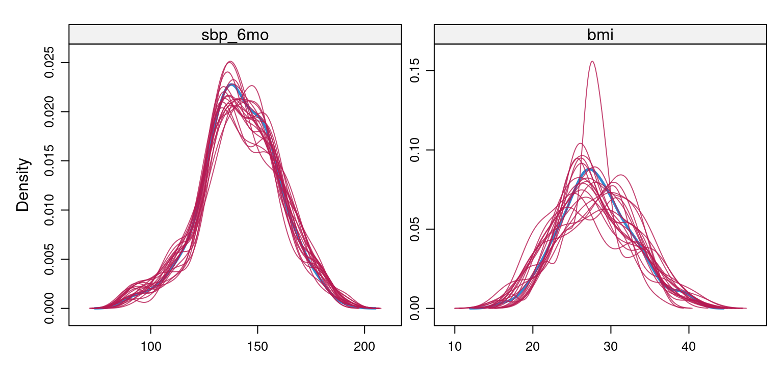
densityplot() overlays the density of observed values (blue) against the imputed values (red, one line per imputation)
We want the imputed distributions to be broadly consistent with the observed distribution in location and shape

Code

densityplot(imp, ~ sbp_6mo + bmi)

Some differences between observed and imputed distributions are expected under MAR. If missingness depends on covariates, the imputed values may reasonably have a different distribution than the observed values
What is concerning: implausible values (e.g., negative BMI), extreme skewness in imputations, or wildly different shapes across imputations

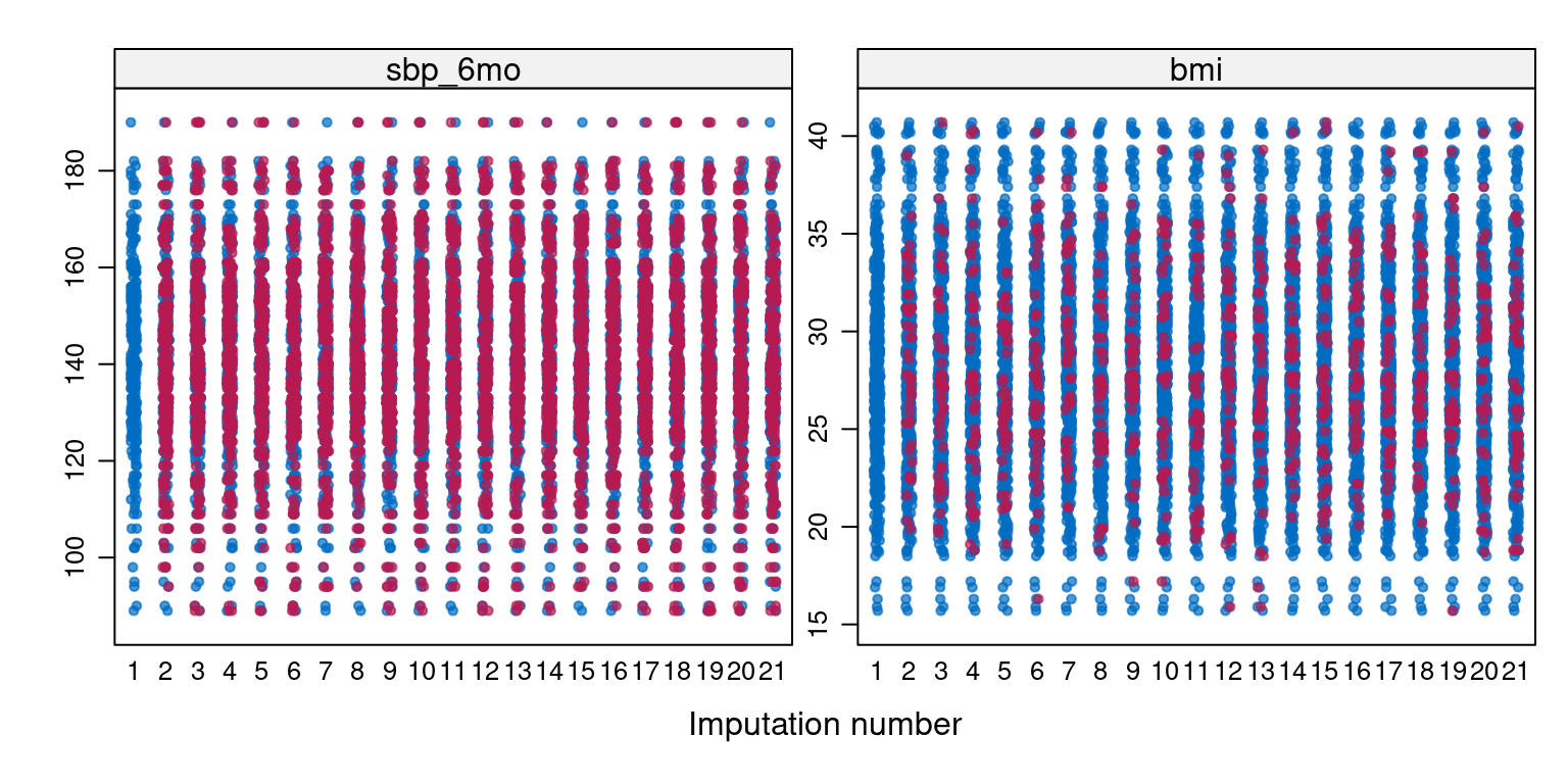
7.2 Strip Plots

stripplot() shows individual imputed values alongside observed values
- Imputation 0 = observed data; imputations 1 through \(m\) = imputed values
- Useful for spotting individual implausible imputations

Code

stripplot(imp, sbp_6mo + bmi ~ .imp, pch = 20, cex = 0.8)

7.3 Scatterplots

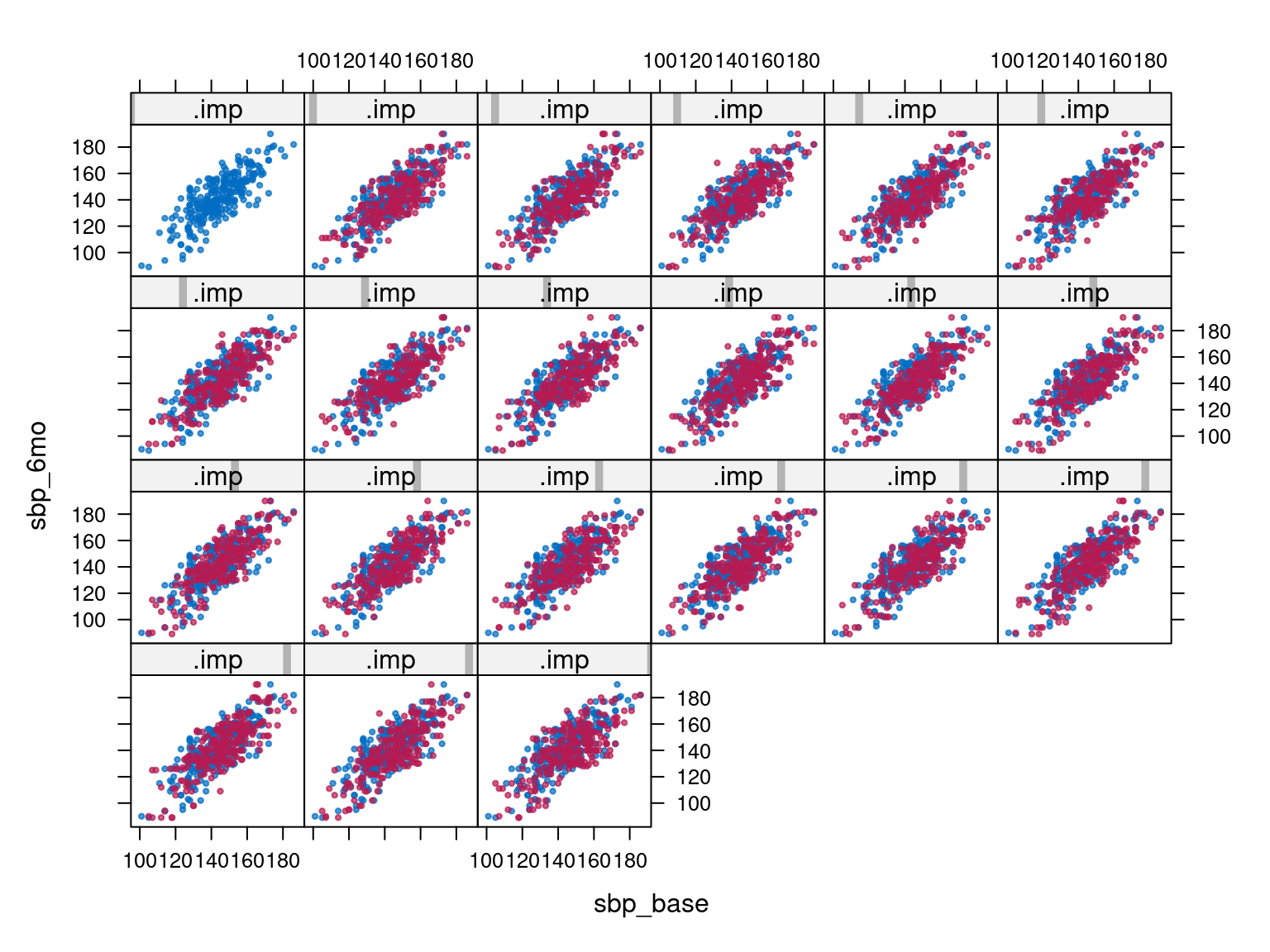
xyplot() shows bivariate relationships, with observed and imputed values distinguished by color
Check that imputed values respect the relationship between variables

Code

xyplot(imp, sbp_6mo ~ sbp_base | .imp, pch = 20, cex = 0.6)

8 Convergence

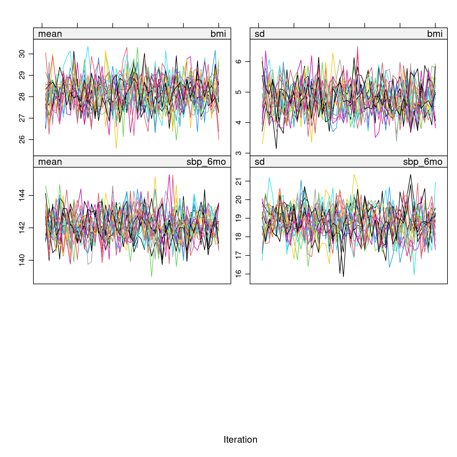
MICE is an iterative algorithm, and convergence must be assessed
At each iteration, the conditional models are re-estimated and imputed values updated
After sufficient iterations, the distribution of imputed values should stabilize
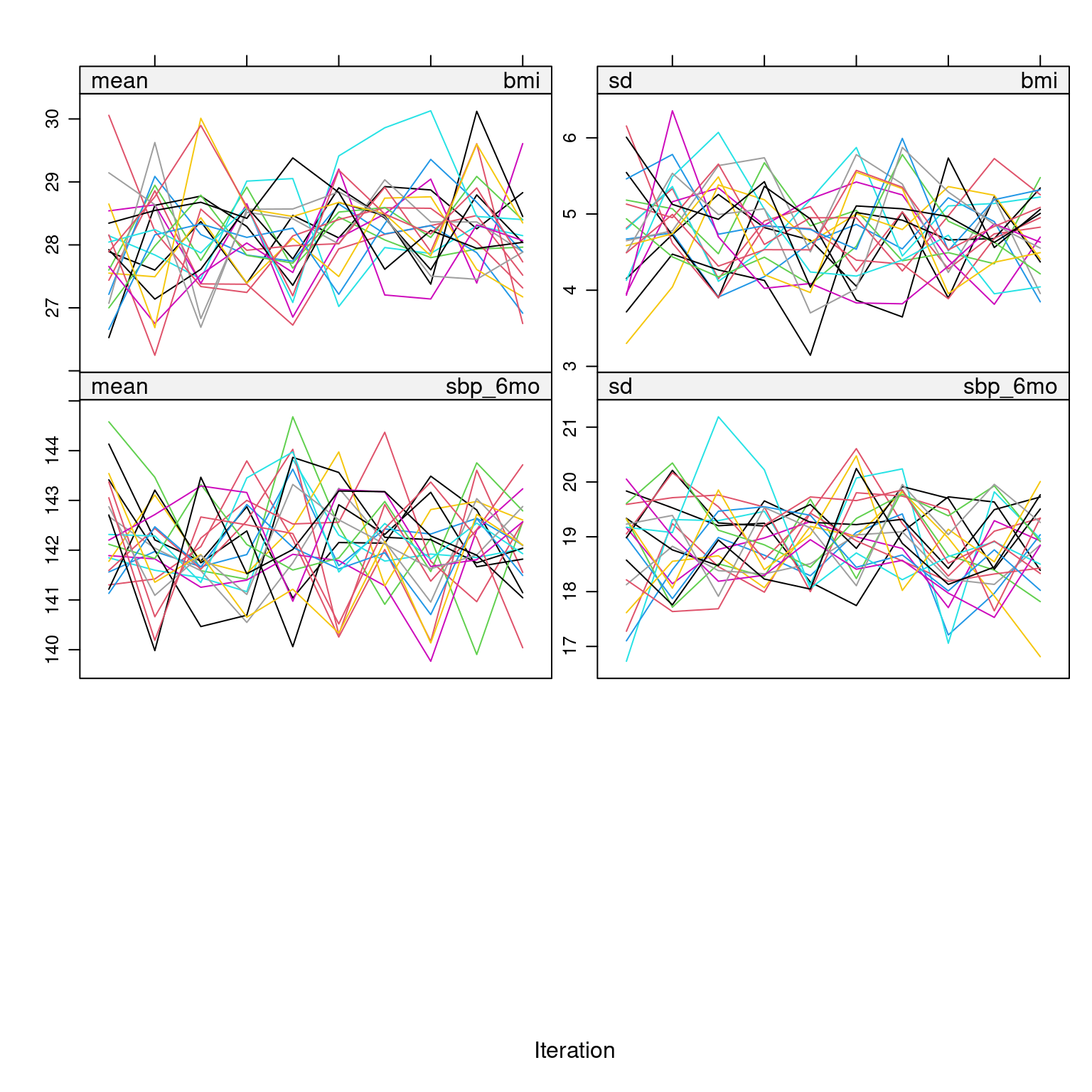
plot() applied to a mids object produces trace plots of the mean and standard deviation of imputed values across iterations, with one line per chain (imputation)

Code

plot(imp)

What to look for:
- Good convergence: Lines are freely intermingled with no systematic trend. The traces resemble white noise or “hairy caterpillars”
- Poor convergence: Trends, drifts, or separation between chains
If convergence appears poor, increase maxit and re-examine

Code

## Run with more iterations to illustrate
imp_long <- mice(dat, m = 20, maxit = 50, seed = 12345, print = FALSE)
plot(imp_long)

9 Analysis and Pooling

9.1 The MI Workflow

The analysis of multiply imputed data proceeds in three steps:
1. Fit the analysis model to each imputed dataset using with()
2. Pool the results across imputations using pool(), which applies Rubin’s rules
3. Summarize the pooled results using summary()

Code

## Step 1: Fit the model to each imputed dataset
fit_mi <- with(imp, lm(sbp_6mo ~ treatment + age + sex + bmi + sbp_base))

## Step 2: Pool using Rubin's rules
pooled <- pool(fit_mi)

## Step 3: Summarize
summary(pooled, conf.int = TRUE) |>
  kable(digits = 4) |>
  kable_styling(bootstrap_options = "striped", full_width = FALSE)

term	estimate	std.error	statistic	df	p.value	2.5 %	97.5 %	conf.low	conf.high
(Intercept)	-12.4287	8.1976	-1.5161	69.3795	0.1340	-28.7809	3.9235	-28.7809	3.9235
treatment	-7.9289	1.2574	-6.3058	59.4490	0.0000	-10.4445	-5.4132	-10.4445	-5.4132
age	0.2184	0.0686	3.1830	50.7909	0.0025	0.0806	0.3561	0.0806	0.3561
sex	-0.3210	1.2112	-0.2650	68.4375	0.7918	-2.7377	2.0957	-2.7377	2.0957
bmi	-0.0022	0.1177	-0.0191	100.7539	0.9848	-0.2358	0.2313	-0.2358	0.2313
sbp_base	1.0100	0.0427	23.6645	59.1298	0.0000	0.9246	1.0954	0.9246	1.0954

9.2 Rubin’s Rules

The pooled estimate \(\bar{Q}\) is the average of the \(m\) individual estimates: \[\bar{Q} = \frac{1}{m} \sum_{i=1}^{m} \hat{Q}_i\]
The pooled variance combines within-imputation variance \(\bar{U}\) and between-imputation variance \(B\): \[T = \bar{U} + \left(1 + \frac{1}{m}\right) B\] where \[\bar{U} = \frac{1}{m} \sum_{i=1}^{m} U_i, \qquad B = \frac{1}{m-1} \sum_{i=1}^{m} (\hat{Q}_i - \bar{Q})^2\]
The factor \((1 + 1/m)\) accounts for using a finite number of imputations
Inference is based on a \(t\)-distribution with degrees of freedom adjusted for the fraction of missing information

9.3 Fraction of Missing Information

The fraction of missing information (FMI) quantifies how much the missing data contribute to the uncertainty of each parameter estimate
- FMI near 0: The estimate is driven by observed data; missing data contribute little additional uncertainty
- FMI near 1: Uncertainty is dominated by the missing data
FMI is useful for assessing whether the number of imputations \(m\) is sufficient

Code

pooled

Class: mipo    m = 20 
         term  m      estimate         ubar            b            t dfcom
1 (Intercept) 20 -12.428712339 3.688569e+01 2.887140e+01 67.200657696   494
2   treatment 20  -7.928851280 8.010450e-01 7.428394e-01  1.581026301   494
3         age 20   0.218388373 2.170879e-03 2.415727e-03  0.004707393   494
4         sex 20  -0.320986056 7.999149e-01 6.353859e-01  1.467070109   494
5         bmi 20  -0.002247722 8.892001e-03 4.729032e-03  0.013857484   494
6    sbp_base 20   1.010027601 9.202168e-04 8.585399e-04  0.001821684   494
         df       riv    lambda       fmi
1  69.37950 0.8218627 0.4511112 0.4662782
2  59.44904 0.9737048 0.4933386 0.5095650
3  50.79094 1.1684271 0.5388362 0.5559828
4  68.43753 0.8340328 0.4547535 0.4700185
5 100.75392 0.5584213 0.3583250 0.3706942
6  59.12976 0.9796244 0.4948537 0.5111147

9.4 Comparison to Truth and Ad Hoc Methods

Code

results_all <- data.frame(
  Method    = c("Truth (complete data)", "Complete case*",
                "LOCF*", "Mean imputation*",
                "IPW (naive SE)", "IPW (sandwich SE)", "IPW (bootstrap SE)",
                "Multiple imputation"),
  Estimate  = c(coef(fit_true)["treatment"],
                coef(fit_cc)["treatment"],
                coef(fit_locf)["treatment"],
                coef(fit_mean)["treatment"],
                coef(fit_ipw)["treatment"],
                coef(fit_ipw)["treatment"],
                coef(fit_ipw)["treatment"],
                summary(pooled)$estimate[
                  summary(pooled)$term == "treatment"]),
  SE        = c(coef(summary(fit_true))["treatment", "Std. Error"],
                coef(summary(fit_cc))["treatment", "Std. Error"],
                coef(summary(fit_locf))["treatment", "Std. Error"],
                coef(summary(fit_mean))["treatment", "Std. Error"],
                coef(summary(fit_ipw))["treatment", "Std. Error"],
                ipw_robust["treatment", "Std. Error"],
                se_boot,
                summary(pooled)$std.error[
                  summary(pooled)$term == "treatment"])
)

results_all |>
  kable(digits = 4, row.names = FALSE,
        caption = "* denotes ad hoc method") |>
  kable_styling(bootstrap_options = "striped", full_width = FALSE)

* denotes ad hoc method
Method	Estimate	SE
Truth (complete data)	-8.2757	0.8779
Complete case*	-8.5101	1.3115
LOCF*	-3.8665	0.7536
Mean imputation*	-4.2115	1.0216
IPW (naive SE)	-8.1456	1.3107
IPW (sandwich SE)	-8.1456	1.3745
IPW (bootstrap SE)	-8.1456	1.3349
Multiple imputation	-7.9289	1.2574

No method exactly recovers the true treatment effect. This is expected, since any method applied to a single dataset with missing values is working with less information than the complete data
The ad hoc methods (complete case, LOCF, mean imputation) show varying degrees of attenuation in the point estimate, and their standard errors do not properly account for the information loss due to missingness
- LOCF and mean imputation can produce artificially small SEs because they treat imputed values as if they were observed, giving a false sense of precision
IPW and MI both produce point estimates closer to the truth
- IPW standard errors are similar across the naive, sandwich, and bootstrap variants in this example because the weights are well-behaved and the missingness model is correctly specified. In practice, with higher missingness rates, more extreme weights, or a less well-specified missingness model, these can diverge substantially
MI produces the smallest SE among the principled methods
- IPW discards the incomplete observations and compensates by upweighting the observed cases. MI uses the predictive relationships among all variables to fill in the missing values, effectively borrowing strength from the observed covariates
- This recovered information translates directly into tighter standard errors
- The MI SE is still larger than the complete-data SE, which is correct. Rubin’s rules appropriately inflate the SE to reflect the additional uncertainty introduced by imputation

10 The `Hmisc`/`rms` Approach

The Hmisc package provides aregImpute(), an alternative imputation engine
- Uses predictive mean matching with optional additive regression (restricted cubic splines and categorical variable transformations)
- Automatically incorporates nonlinear relationships in the imputation model
The rms package provides fit.mult.impute(), which fits an rms model (e.g., ols, lrm, cph) to the multiply imputed data and pools the results using Rubin’s rules

Code

library(Hmisc)
library(rms)

set.seed(12345)
areg_imp <- aregImpute(~ treatment + age + sex + bmi + sbp_base +
                          side_effects + sbp_6mo,
                        data = dat,
                        n.impute = 20,
                        nk = 3)

Iteration 1 
Iteration 2 
Iteration 3 
Iteration 4 
Iteration 5 
Iteration 6 
Iteration 7 
Iteration 8 
Iteration 9 
Iteration 10 
Iteration 11 
Iteration 12 
Iteration 13 
Iteration 14 
Iteration 15 
Iteration 16 
Iteration 17 
Iteration 18 
Iteration 19 
Iteration 20 
Iteration 21 
Iteration 22 
Iteration 23

Code

areg_imp


Multiple Imputation using Bootstrap and PMM

aregImpute(formula = ~treatment + age + sex + bmi + sbp_base + 
    side_effects + sbp_6mo, data = dat, n.impute = 20, nk = 3)

n: 500  p: 7    Imputations: 20     nk: 3 

Number of NAs:
   treatment          age          sex          bmi     sbp_base side_effects 
           0            0            0           47            0            0 
     sbp_6mo 
         228 

             type d.f.
treatment       l    1
age             s    2
sex             l    1
bmi             s    2
sbp_base        s    2
side_effects    l    1
sbp_6mo         s    1

Transformation of Target Variables Forced to be Linear

R-squares for Predicting Non-Missing Values for Each Variable
Using Last Imputations of Predictors
    bmi sbp_6mo 
  0.055   0.723

Code

dd <- datadist(dat)
options(datadist = "dd")

fit_areg <- fit.mult.impute(sbp_6mo ~ treatment + age + sex + bmi + sbp_base,
                            fitter = ols,
                            xtrans = areg_imp,
                            data = dat)


Wald Statistic Information

Variance Inflation Factors Due to Imputation:

Intercept treatment       age       sex       bmi  sbp_base 
     1.67      2.17      1.20      1.32      1.63      2.01 

Fraction of Missing Information:

Intercept treatment       age       sex       bmi  sbp_base 
     0.40      0.54      0.16      0.24      0.38      0.50 

d.f. for t-distribution for Tests of Single Coefficients:

Intercept treatment       age       sex       bmi  sbp_base 
   118.57     65.24    707.40    323.02    128.21     75.30 

The following fit components were averaged over the 20 model fits:

  fitted.values stats linear.predictors

Code

fit_areg

Linear Regression Model

fit.mult.impute(formula = sbp_6mo ~ treatment + age + sex + bmi + 
    sbp_base, fitter = ols, xtrans = areg_imp, data = dat)

                 Model Likelihood    Discrimination    
                       Ratio Test           Indexes    
Obs      500    LR chi2    600.56    R2       0.699    
sigma10.1742    d.f.            5    R2 adj   0.696    
d.f.     494    Pr(> chi2) 0.0000    g       17.354    

Residuals

     Min       1Q   Median       3Q      Max 
-59.2104  -5.8900  -0.1495   6.4232  28.8601 

          Coef     S.E.   t     Pr(>|t|)
Intercept -11.7255 8.0209 -1.46 0.1444  
treatment  -7.8849 1.3530 -5.83 <0.0001 
age         0.2051 0.0523  3.92 0.0001  
sex        -0.4292 1.0541 -0.41 0.6841  
bmi        -0.0100 0.1229 -0.08 0.9351  
sbp_base    1.0124 0.0441 22.95 <0.0001

fit.mult.impute() returns an rms fit object, so all standard rms tools apply:
- summary() for effect estimates and confidence intervals
- anova() for chunk tests
- Predict() for adjusted predictions
- nomogram() for clinical prediction tools

11 Practical Considerations

11.1 Number of Imputations

The traditional recommendation of \(m = 5\) imputations dates to an era when computation was expensive
Modern guidance (e.g., White et al., 2011) suggests that \(m\) should be at least as large as the percentage of incomplete cases
- If 25% of observations have at least one missing value, use \(m \geq 25\)
Too few imputations lead to:
- Unstable pooled estimates (especially for \(p\)-values and confidence intervals)
- Poor reproducibility across different random seeds
With modern computing, there is little reason not to use \(m = 20\) or more as a default

11.2 Auxiliary Variables

Auxiliary variables are variables that are:
- Predictive of the missing values, or
- Predictive of the probability of missingness, or
- Both
Including auxiliary variables in the imputation model strengthens the plausibility of the MAR assumption and can improve the efficiency of MI estimates
Auxiliary variables do not need to appear in the analysis model
- For example, a lab value that predicts dropout but is not part of the scientific question can still be included in the imputation model
Excluding relevant auxiliary variables is a common and consequential mistake
- It weakens the MAR assumption and can introduce bias

11.3 Including the Outcome

The outcome variable should always be included in the imputation model, even when only covariates are missing
Omitting the outcome from the imputation model leads to imputed covariate values that do not reflect the covariate-outcome relationship
- This attenuates regression coefficients in the analysis model
This is counterintuitive because it feels like “using the outcome to predict covariates,” but it is necessary for valid MI

11.4 Congeniality

The imputation model should be at least as rich as the analysis model
- If the analysis model includes an interaction (e.g., treatment \(\times\) sex), the imputation model should include that interaction as well
- If the analysis model includes nonlinear terms (e.g., restricted cubic splines for age), the imputation model should accommodate nonlinearity
An imputation model that is less flexible than the analysis model is called uncongenial
- Uncongeniality can bias the analysis results and invalidate the pooled standard errors
In practice, it is safer to make the imputation model somewhat more flexible than the analysis model rather than less flexible

11.5 The MAR Assumption

All of the MI methods described in these notes assume the data are MAR
MAR means that the probability of missingness depends on observed data but not on the missing values themselves, after conditioning on the observed data
MAR cannot be verified from the data
- Little’s MCAR test can reject MCAR, but it cannot distinguish MAR from MNAR
- If MNAR holds, MI under MAR will generally produce biased estimates
When MNAR is a concern, sensitivity analyses can assess how robust the conclusions are to departures from MAR
- These methods require careful specification informed by domain knowledge about the mechanism of missingness

11.6 Parallel Computing

For large datasets or complex imputation models, the MICE algorithm can be slow
The mice package supports parallel computation via futuremice(), which distributes the \(m\) imputations across multiple processor cores
Each imputation is independent, so parallelization is straightforward

Code

library(future)
library(furrr)

plan(multisession, workers = 4)
imp_par <- futuremice(dat, m = 20, maxit = 10, seed = 12345, n.core = 4)

This is most beneficial when the dataset is large or the number of imputations is large (e.g., \(m \geq 50\))
For most biostatistical applications with moderate sample sizes, the sequential default is fast enough

12 References

van Buuren, S. (2018). Flexible Imputation of Missing Data (2nd ed.). Chapman & Hall/CRC. Freely available at https://stefvanbuuren.name/fimd/
van Buuren, S. and Groothuis-Oudshoorn, K. (2011). mice: Multivariate Imputation by Chained Equations in R. Journal of Statistical Software, 45(3), 1–67.
Rubin, D. B. (1987). Multiple Imputation for Nonresponse in Surveys. New York: Wiley.
White, I. R., Royston, P., and Wood, A. M. (2011). Multiple imputation using chained equations: Issues and guidance for practice. Statistics in Medicine, 30(4), 377–399.
Carpenter, J. R. and Kenward, M. G. (2013). Multiple Imputation and Its Application. Wiley.
Harrell, F. E. (2015). Regression Modeling Strategies (2nd ed.). Springer. See Chapter 3 for discussion of missing data and multiple imputation.

1 Introduction

2 Setup and Data

2.1 A Synthetic Clinical Trial Dataset

3 Exploring and Characterizing Missingness

3.1 Missing Data Patterns

3.2 Visualizing Missingness

3.3 Comparing Observed Characteristics by Missingness Status

3.4 Little’s MCAR Test

3.5 Margin Plots

4 Ad Hoc Methods: A Demonstration

4.1 The True Treatment Effect

4.2 Complete Case Analysis

4.3 Last Observation Carried Forward (LOCF)

4.4 Mean Imputation

4.5 Comparison of Ad Hoc Methods

5 Inverse Probability Weighting

5.1 Overview

5.2 Implementation

5.2.1 Sandwich Standard Errors

5.2.2 Bootstrap Standard Errors

5.2.3 Comparing IPW Standard Errors

5.3 Limitations of IPW

6 Multiple Imputation with mice

6.1 The MICE Algorithm

6.2 Running mice()

6.3 The Methods Vector

6.4 The Predictor Matrix

7 Imputation Diagnostics

7.1 Density Plots

7.2 Strip Plots

7.3 Scatterplots

8 Convergence

9 Analysis and Pooling

9.1 The MI Workflow

9.2 Rubin’s Rules

9.3 Fraction of Missing Information

9.4 Comparison to Truth and Ad Hoc Methods

10 The Hmisc/rms Approach

11 Practical Considerations

11.1 Number of Imputations

11.2 Auxiliary Variables

11.3 Including the Outcome

11.4 Congeniality

11.5 The MAR Assumption

11.6 Parallel Computing

12 References

6 Multiple Imputation with `mice`

6.2 Running `mice()`

10 The `Hmisc`/`rms` Approach